BE01106 Business Statistics Assignment

Introduction

The Assignment Data (PopulationPropertyData.xls) file, which you can access from the Assessment Information page on the unit website contains, in the range A1:I401, real estate sales data for a population of 400 properties around Melbourne in a particular week. You are required to select a random sample of 50 properties from this population. The variables in the data set are as follows:

{`
  V1 = Region where property is located (1 = North, 2 = West, 3 = East, 4 = Central)
  V2 = Property type (0 = Unit, 1 = House)
  V3 = Sale result (1 = Sold at auction, 2 = Passed-in, 3 = Private sale, 4 = Sold before auction).
  Note that a blank cell for this variable indicates that the property did not sell.
  V4 = Building type (1 = Brick, 2 = Brick veneer, 3 = Weatherboard, 4 = Vacant land)
  V5 = Number of rooms
  V6 = Land size (Square metres)
  V7 = Sold Price ($000s)
  V8 = Advertised Price ($000s)
  Column A (PN), contains the property identification numbers from 001 to 400 properties.
  `}

Selecting your Random Sample and Creating your Sample Data File

To select your random sample, you need:

A printed copy of the Random Number Table handy.
Open the PopulationPropertyData.xls file on computer screen.
Create a SamplePropertyData Excel file and keep it open on computer screen.

In order to select the sample data that will form the basis of your assignment you will need to make use of the random number table provided as a pdf file (RandomNumbers.pdf) on the Assessment Information page of the unit website. The provided table of random numbers is, as the title suggests, a sequence of randomly generated numerical digits (0 to 9). These digits are arranged in a table with ten columns (numbered 0 to 9) and one hundred rows (numbered 01 to 00) spread over two pages. The entries in each column of each row consist of six single digits.

Your first task is to select 50 three-digit random (property) numbers ranging from 001 to 400 from the table of random numbers. The type of simple random sampling that we will be engaged in here is termed “without replacement” because we specifically do not want to allow a property number to be selected more than once. If we allowed this to occur we would run the risk of the sample being biased and so not representative of the population. In the population, a particular property only occurs once and so it would not do to allow a particular property to occur more than once in your sample. In this way we can be more assured that the sample is typical of the population and so perform inferential statistical analyses about the population with some confidence.

In order to select your 50 random property numbers you will need to first go to a starting position row and column in the random number table (Note ~ not the population property data) defined by the last three digits of your VU student identification number (the assignment marker will check your student ID number against the three digits number you use to collect the random sample). The last two digits of your VU ID number identifies the row and the third last digit identifies the column of your (relatively) “unique” starting position.

For demonstration purposes, if the last three digits of your student identification were 7, 4 and 9 (i.e. 749), you would commence your property number selection at the starting position - row 49 and column 7 of the random number table. You are required to colour/highlight the starting row number 49 and the starting column number 7. You should be able to see that the six digit number occupying that position is 217035.

Then, moving across the row, from left to right from the starting position, examine the first three digits of each six digit number and then the second three digits in each of the columns of the table. If any of these three digit numbers are between 001 to 400 inclusive, they are “good” numbers (the population data numbered from 001 to 400). Ignore any number greater than 400 or equal to 000. They are “not-good” numbers

Continue reading across row 49 from left to right starting at column 7 as instructed, you would encounter the following three digit good numbers:

217, 035, 306, 150, …

You need to record the first good property numbers, i.e. 217, and open the PopulationPropertyData.xls Excel file located on the Assessment Information page of the unit website. On the spreadsheet, scroll down the PN column to locate 217 (note: do not select the Excel spreadsheet row number 217. Select the row with 217 in the PN column). At this row, highlight from 217 under the PN column across to the right up to the V8 column, use Cut and Paste procedure to cut the row of data and paste the data into a new Excel file (name it and save it as SamplePropertyData.xlsx). Next is to repeat the Cut and Paste process for PN 035, and for PN 306 and the subsequent three digit good numbers selected from Random Number Table up to the point when the row of the spreadsheet in the SamplePropertyData file grown up to 50 rows of data. Make sure you copy the column headings, PN, V1, ... V8 into your sample data file as the heading for the columns.

Each time a number is selected from the Random Number Table, insert a strikethrough mark over the selected number on the Random Number Table to mark it off. It is possible that you may come across some three digit good numbers more than once (we call them “repeated” number). The use of the Cut and Paste procedure is the “without replacement” sampling procedure to ensure that no repeated PN number and the corresponding data can be select more than once in this sample selection process. When a repeated number is found, colour/highlight/cross-out it in the Random Number Table to indicate that this good number has not been used to select the sample data (See the Assignment Part I Model Answers file).

Note that if you reach to the end of Row 50 on the first page of the Random Number Table but still not yet to collect 50 good numbers, continue the process on to Row 51 on the top of the second page of the Random Number Table (as the same practice in the Assignment Part I Model Answer). Similarly if you reach to the end of Row 00 on the second page, proceed on to row 01 on the top of the first page. Once 50 good numbers are selected and the 50 rows of data have been copied from the PopulationPropertyData file into the SamplePropertyData file, this will form a completed sample data set occupying spreadsheet columns A to I and spreadsheet rows 1 to 51 (Refer to the Assignment Part I Model Answers file on the Assessment Information).

Assignment Part I

Part I of the assignment simply requires the submission of a hard copy of your sample property data presented in a maximum of no more than 3 printed pages in total. (See the Assignment Part I Model Answer). This sample data set will form the basis of the statistical presentation and analysis tasks contained in Part II of the assignment.

Task 1

Make a hard copy of your Random Number Table containing the following:
1. The highlight of the starting row and starting column of the sample selection process. (Refer to the Assignment Part I Model Answer).
2. The strikethrough/mark on the three digits good numbers and the cross-out of the repeated number(s). (Refer to the Assignment Part I Model Answer).
Print a hard copy (see note below) of your sample property data (9 columns x 51 rows of data plus the column headings row) from the Excel file (SamplePropertyData) obtained per the above instructions.

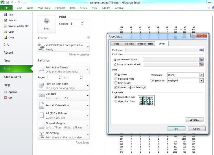
Note: when printing the hard copies in (b) please select Page Setup in Excel and then under Print in the Sheet window, tick the Gridlines and Row and column headings check boxes. This will ensure that the Excel row and column headings are included in your Excel printout. The screenshot for printing row and column heading is attached below for reference.

BE01106 Business Statistics Assignment image 1

Assignment Part II

Answers to the six assignment tasks in Part II must be based on the sample data file that you have created in Part I. All tasks in this assignment require you to obtain an Excel output prior to performing some analysis. Copy and Paste these outputs to your assignment MS- Word document immediately preceding any subsequent analysis. Explanations must be precise and to the point. Charts and tables must have appropriate titles and numerical values must be rounded to an appropriate number of decimal places and accompanied by the correct units of measure.

Task 2

Use Excel to produce a Frequency Column Chart and a Relative Frequency Pie-Chart for your sample to show the number and proportion, respectively, of each building type.

Use these graphical summaries to answer the following questions:

How many properties in your sample consist of brick buildings?
Which building type occurs most frequently in your sample?
What proportion of properties in your sample consists of weatherboard buildings?

Task 3

Use Excel to sort your sample “Sold Price” data and paste into your MS Word assignment document.
Use the percentile location formula;
L_P =(n+1) * p/100, and the three associated rules (Slide 11 of Week 2 Seminar, Session 1) to determine:
1. The 70^th percentile.
2. The first and third quartiles.
Briefly explain what the 70^th percentile that you have determined informs you about your sample “Sold Price” data.
Determine the Inter-Quartile Range of your sample “Sold Price” data and provide a brief explanation of what information this statistic provides about your sample data.

Task 4

Use Excel to produce a Descriptive Statistics table for your sample “Sold Price” data and paste into your MS Word assignment document.
Use results from Task 3 to determine manually for this data, the upper and lower inner fence limits;
IFUL = Q3 + 1.5 x IQR
and IFLL = Q1 – 1.5 x IQR
Based on the limits calculated in (b), choose from the numerical summary measures provided in the Descriptive Statistics table, and/or measures calculated previously in Task 3;
1. an appropriate measure of central tendency, and,
2. an appropriate measure of dispersion for your sample “Sold Price” data.

Provide a brief explanation of the reasoning behind your choice in both cases.

Task 5

From the Descriptive Statistics table obtained in Task 5, identity three pieces of evidence that indicate whether your sample “Sold Price” data has been obtained from a normally distributed population or not. What is your conclusion? Note: Make sure only one piece of evidence relates to the shape of the sample data.
Regardless of your conclusion in above, assume the “Sold Price” population data is normally distributed. Applying the Standard Normal tables, calculate how many “Sold Price” observations in your sample would expect to lie within 1.5 standard deviations of the mean (i.e. between z = –1.5 and z = +1.5).
(c) Use the mean and standard deviation from the Descriptive Statistics table of Task 5 to calculate the bound for 1.5 standard deviation spread from the mean. Using the “Sold Price” sample data, manually count the number of observations fall within the bound. State whether this count matches, approximately, your answer to (b) and hence whether this result confirms (or not) your conclusion in (a).

Task 6

Use Excel to produce a Descriptive Statistics table for the “Sold Price” variable in your sample suitable for constructing an interval estimate of the population mean “Sold Price”. Hence determine:
1. A point estimate of the mean “Sold Price” of the population of properties.
2. A 90% confidence interval estimate of the mean “Sold Price” of the population of properties.
3. Make a brief verbal statement explaining the meaning of the confidence interval estimate obtained in (ii) in the context of the variable in this task.
If the population mean “Sold Price” is actually 650 ($000s), would you consider the interval estimate obtained in (a), to be satisfactory? Explain why or why not.

Task 7

Use Excel to produce a Descriptive Statistics table for the brick veneer properties in your sample suitable for constructing an interval estimate of the population proportion of brick veneer properties. Hence determine:
1. A point estimate of the proportion of brick veneer properties in the population.
2. A 99% confidence interval estimate of the proportion of brick veneer properties in the population.
Using the following formula:
(sample statistic) (critical z or t) (standard error of the sample statistic)
Use the rule of thumb for good normal approximation (Slide 3 of Week 7 Session 2) for proportion, then the Empirical Rule (Slide 8 of Week 5 Session 1) for a Normal distribution to determine a 95% confidence interval estimate of the proportion of brick veneer properties in the population.
Compare, in terms of the precision, the interval manually calculated in (b) with the interval obtained from the Descriptive Statistics table in (a). Explain why the direction of the change in precision is expected.

INSTRUCTIONS FOR OBTAINING EXCEL OUTPUTS FOR Tasks 2 - 4 OF THE BEO1106 ASSIGNMENT.

The following step by step instructions are provided for you so that you are able to obtain the Excel outputs required for completing tasks 2 - 4 of the Business Statistics assignment tasks due in week 8.

Note that the specifics of these instructions, and hence the resulting outputs, refer to a demonstration set of sample data contained in columns A to I, rows 1 to51 (including column headings) of an MS Excel assignment data file. Because of this, the Excel outputs that you obtain using your data will, with almost complete certainty, be different to what you see in the demonstrations that follow.

As you perform the steps for each assignment task make sure you pay particular attention to instructions regarding spreadsheet cell locations, modifying them where necessary to suit your particular data set. This is important so that subsequent work on the assignment flows consistently. Also, make sure that when you conclude an assignment work session you progressively save your spreadsheet work and continue on with the saved file once you recommence work in your next assignment work session.

Note: References to MS Excel and Word in this document are to version 2016 (installed in computer laboratories at VU). For assistance with earlier versions of Excel/Word please see your seminar leader.

Open your Excel file SamplePropertyData.xls which you created after the seminar in week 4. The variables contained in this data file are as follows:

{`
  V1:Region around Melbourne where property is located (1 = North, 2 = West, 3 = East, 4 = Central)
  V2:Property type (0 = Unit, 1 = House)
  V3:Sale result (1 = Sold at auction, 2 = Passed-in, 3 = Private sale, 4 = Sold before auction)
  V4:Building type (1 = Brick, 2 = Brick veneer, 3 = Weatherboard, 4 = Vacant land)
  V5:Number of rooms
  V6:Land size (Square metres)
  V7:Sold Price ($000s)
  V8:Advertised Price ($000s)
  Column A (PN), contains the property identification numbers for the 400 properties.
  `}

Tables, Graphs and Numerical Summaries of Data

Assignment Task 2

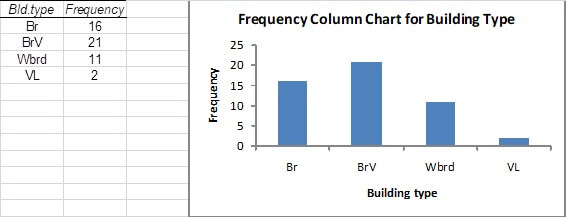
In Task 2 you are required to use Excel to produce a Frequency Column Chart and a Relative Frequency Pie-Chart for your sample to show the number and proportion, respectively, of each building type.

Although the following steps demonstrate how to do this, note that the Excel outputs you obtain will be different to what follows, as you will almost certainly be using different data to that used in this demonstration.

Step 1:

Create a basic frequency table and column chart summary of the “Building type” sample data.

Type the word bins in a cell in any unused column, say for example, J1. In range J2:J5 type the individual “values” of the “Building type” categorical variable, V4, i.e. 1 in cell J2, 2 in cell J3, 3 in cell J4 and 4 in cell J5. From the Data menu (Analysis grouping) select Data Analysis (see the Additional Learning Resources page of the unit website if Data Analysis does not appear under the Analysis grouping on the Data menu). Select Histogram from the Data Analysis Tools list and then select OK.

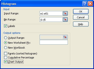
BE01106 Business Statistics Assignment image 2

In the Histogram dialogue box you will need to specify, in the Input Range, the cell locations of the “Building type” variable values i.e. e1:e51, if you wish to include reference to the column heading, “V4”.

You will also need to specify, in the Bin Range, the cell locations of the individual categorical variable “values” that you identified at the beginning of Step 1 i.e. j1:j5, if you wish to include reference to the column heading, “bins”.

Tick the Labels box if the first cells in your Input Range and Bin Range specifications contain column headings (as in this case).

Select New Worksheet Ply (if not specified by default) so that the output will appear on a new worksheet of the MS Excel workbook.

Tick the Chart Output box in order to request a basic frequency table and column chart.

Select OK to obtain the basic frequency table and column chart.

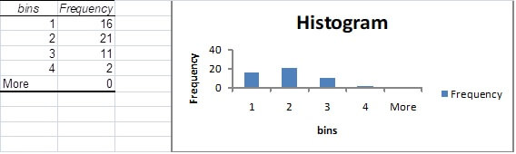
BE01106 Business Statistics Assignment image 3

Note: The frequency table and column chart provided by Excel at this point are very basic and need to be refined so as to provide a more precise and informative summary of the “Building type” data.

Step 2:

Modify the basic frequency table and frequency column chart output provided by Excel to provide a more precise and informative summary of the “Building type” data.

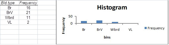
The frequency table should make reference to the variable of interest. We can achieve this, in this case, by typing the (abbreviated) words “Bld. type” over the column heading “bins” in the Excel worksheet.

The categorical “values” 1, 2, 3 and 4 (in this case) in the frequency table should also be changed to the more informative (abbreviated), “Br”, “BrV”, “Wbrd” and “VL” respectively. Note that when you do this, these labels will automatically replace the horizontal axis markings of 1, 2, 3 and 4 on the column chart.

The frequency table contains a row labelled “More” to cover the possibility of “values” in the data set other than 1, 2, 3 and 4. Since there are no such values in this case the “More” row is redundant and can be removed. To do so simply activate the “More” cell and then from the Home menu (Cells grouping) access the Delete drop down menu and select Delete Sheet Rows and the entire row containing the reference to “More” will be deleted from the worksheet. Note that when you do this the marking on the horizontal axis of the column chart specified as “More” will automatically disappear.

BE01106 Business Statistics Assignment image 4

The column chart will also require some modification.

Firstly, note that the graph is incorrectly titled “Histogram”. The word “histogram” should in fact be reserved for the equivalent graphical output for quantitative (or (real) numerical) data. If a title is required for this graphical output a more correct and informative description would be, in this case, “Frequency Column Chart for Building Type”. If you left click on the title “Histogram” you will be able to delete the existing title before replacing it with the more suitable title. You may need to adjust the font size (see Home menu, Font grouping) to make the title more presentable.

Similarly the label for the horizontal axis, “bins”, should be replaced with a more informative descriptive label for the variable of interest (in this case, say, “Building type”).

The legend on the right hand side of the graph (“Frequency”) is largely redundant as the vertical axis is clearly labelled as such. This legend can be deleted by left clicking on it and then pressing the delete key on your keyboard.

You may observe that the column chart is rather flat and has a rather imprecise scale on the vertical axis. If this is the case these aspects can be rectified by left clicking on the white Chart Area around the column chart (within the rectangular border) at which point you should observe small sets of “dot” indicators appear around the perimeter of the border. Clicking on and dragging down the indicators at the centre of the bottom edge of the border will stretch out the column chart vertically and at the same time will increase the graduations along the vertical axis.

BE01106 Business Statistics Assignment image 5

Step 3:

Copy the graphical output into your MS Word assignment document to form part of your completed assignment (Part II).

With the “dot” indicators still observable around the perimeter of the chart area border (left click on the white Chart Area if this is not the case), select the Copy () icon from the Home menu (Clipboard grouping).

Open your MS Word document and then select the Paste () icon from the Home menu (Clipboard grouping) to insert the column chart into the document.

Step 4:

Create a basic (relative frequency) pie chart summary of the “Building type” sample data.

In MS Excel right click anywhere inside the Chart Area of the column chart you have just constructed and then select Change Chart Type from the pop-up menu.

From the Change Chart Type Templates list select Pie and then OK to convert your frequency column chart into a basic relative frequency pie chart.

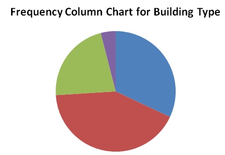
BE01106 Business Statistics Assignment image 6

Note: The pie chart provided by Excel at this point may be incorrectly titled (in this case “Frequency Column Chart …”) and is lacking in important detail (in particular the category labels and relative frequencies corresponding to each sector).

Step 5:

Modify the basic (relative frequency) pie chart output provided by Excel to provide more detail and clarity of presentation.

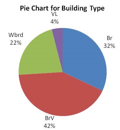
An incorrect or inappropriate title can be rectified by left clicking on it (as for the Column Chart) and replacing it with a more appropriate description (perhaps “Pie Chart for Building Type” in this case).

More detail can be provided (in the form of actual relative frequencies for each of the categories as well as accompanying descriptive labels) by right clicking anywhere inside the “pie” and selecting Add Data Labels from the pop-up menu (at which point frequency counts for each category will appear in the sectors of your pie chart).

To obtain relative frequency (%) information relating to the various categories right click again anywhere inside the “pie” and select Format Data Labels from the pop-up menu to show the Format Data Labels dialogue box.

In the Format Data Labels list of Label Options tick the Category Name and Percentage boxes and whatever Label Position (perhaps Outside End) you prefer.

Select Close to obtain the improved relative frequency pie chart.

BE01106 Business Statistics Assignment image 7

Note: If your pie chart is “flat” you can stretch it out by repeating the procedure described at the end of Step 2 for the column chart.

Step 6:

Copy the graphical output into your MS Word assignment document to form part of your completed assignment (Part II).

Left click on the white Chart Area (at which point the “dot” indicators will appear around the perimeter of the border) and then select the Copy icon from the Home menu.

Open your MS Word document and then select the Paste icon from the Home menu to insert the pie chart into the document.

Assignment Task 3

In Task 3 you are required to use MS Excel to sort the “Sold Price” data in your sample as a preliminary to manually determining percentile information for that data.

Step 1:

Sort the “Sold Price” sample data into ascending order.

With your Excel workbook open at the sample data worksheet, click on cell H2 and then drag to highlight the entire contents of column H, rows 2 to 51.

From the Home menu select the Copy icon and then paste the contents of cells H2 to H51 into any unused column, say, M1 to M50 (by activating cell M1 and the selecting the Paste icon).

With cells M1 to M50 highlighted, from the Data menu, Sort and Filter grouping, select the Sort Smallest to Largest (A to Z or Z to A) icon at which point the original contents of cells M1 to M50 will be sorted into ascending order (with any blank cells, indicating that the property did not sell, appearing at the bottom).

For the data that forms the basis of this demonstration there were five missing “Sold Price” values resulting in the sorted data occupying cells M1 to M45 (and 5 blank cells appearing in cells M46 to M50).

Step 2:

Copy the sorted column of “Sold Price” sample data into a suitable number of smaller columns (say five in this case) in your Excel worksheet as a prelude to a more manageable transferral of the sorted data into a Word document.

Highlight cells M1 to M10 and then select the Copy icon (from the Home menu).

Activate an empty cell (say N1) which can be imagined to form the top left hand corner of an empty block of five columns and ten rows stretching from cell N1 to R10.

Select Paste from the Home menu to transfer a copy of the first ten sorted “Sold Price” data into cells N1 to N10.

The second group of ten sorted “Sold Price” data can now be copied into cells O1 to O10 by first highlighting cells M11 to M20 and repeating the “copy/paste” process just performed (you will have to activate cell O1 before you perform the “paste” operation).

Repeating this process three more times will produce a copy of the sorted “Sold Price” sample data into a block of up to five columns and ten rows (from cell N1 to R10).

For the data that forms the basis of this demonstration, the 45 sorted “Sold Price” values occupied the block of almost five complete columns of ten rows from cell N1 to R5.

Step 3:

Copy the more manageable block of sorted “Sold Price” sample data into a MS Word document to form part of your completed assignment.

Highlight the sorted data in columns N to R and then select the Copy icon from the Home menu to facilitate the “pasting” of the block of up to five columns and ten rows into your Word document.

Assignment Task 4

In Task 4 you are required to use Excel to produce a Descriptive Statistics table for the “Sold Price” data in your sample.

Step 1:

Obtain a descriptive statistics table for the “Sold Price” sample data.

With your Excel workbook open at the sample data worksheet select Data Analysis from the Data menu.

Select Descriptive Statistics from the Data Analysis Tools list and then select OK.

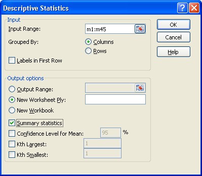
BE01106 Business Statistics Assignment image 8

In the Descriptive Statistics dialogue box you will need to specify, in the Input Range, the cell locations of the sample “Sold Price” variable values. This will be most easily achieved from column M after the sorting process of Step 1 of Task 4 above. For the data that forms the basis of this demonstration the locations are M1:M45.

Grouped By: Columns needs to be selected (if not already by default) to indicate that the data set for which numerical summaries are required is contained in a column (rather than a row).

We will NOT tick the Labels in First Row box on this occasion since the first cell in the Input Range, M1, does not contain a column heading.

Select New Worksheet Ply (if not already by default) so that the output will appear on a new worksheet of the MS Excel workbook.

Tick the Summary statistics box to obtain a comprehensive set of numerical summaries.

Select OK to obtain the basic descriptive statistics table.

BE01106 Business Statistics Assignment image 9

Note: The descriptive statistics table provided by Excel at this point is a little raw with regard to the information it provides and needs to be modified so as to provide a more informative summary of the “Sold Price” sample data.

Step 2:

Modify the basic descriptive statistics table output provided by Excel to provide a more informative summary.

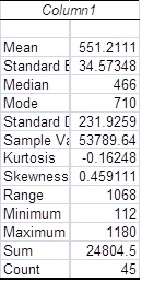
The most obvious deficiency of the initial table provided by Excel is that the table does not make explicit reference to the variable of interest (including units). In this case the heading “Column1” is completely inadequate. This can be rectified by replacing it with “Sold Price ($000)”.

Note also that the left hand column is so narrow that it has truncated some of the descriptions relating to the particular numerical summaries provided. Expanding the column until all descriptions are visible in full will overcome this problem. Alternatively (or in addition) lengthy descriptors could be replaced by abbreviations that still clearly identify the numerical summary concerned (e.g. Std. Deviation for Standard Deviation).

The number of decimal places quoted in the descriptive statistics table should reflect the data being summarised and/or the particular summary under consideration. Generally, numerical summaries measured in the same units as the original data should contain no more than one or two decimal places more than that contained in the raw data. So, in this case, with V7 often being recorded to one decimal place, two or three decimal places would be more than enough for most of the numerical summaries provided in the descriptive statistics table. For our purposes measures such as kurtosis and skewness will not require any more than two-decimal place accuracy.

Taking consideration of the accuracy issues raised above, for the “Sold Price” descriptive statistics table, the numerical contents of cells B3, B4, B7 and B8 could be rounded to three decimal places by clicking on the cell (or groups of cells) and then clicking on the Decrease Decimal icon in the Number grouping of the Home menu until the required number of decimal places is obtained. Similarly the contents of cells B9 and B10 could be rounded to two decimal places.

As a result of the modifications referred to above the improved “Sold Price” descriptive statistics table appears as:

Sold Price ($000)
Mean	551.211
Standard Error	34.573
Median	466
Mode	710
Std. Deviation	231.926
Sample Variance	53789.642
Kurtosis	-0.16
Skewness	0.46
Range	0.46
Minimum	112
Maximum	1180
Maximum	1180
Sum	24804.5
Count	45

Step 3:

Copy the descriptive table into your MS Word assignment document to form part of your completed assignment.

Left click on cell A1 of the descriptive statistics table and then drag to highlight the entire contents of columns A and B. Then select the Copy icon from the Home menu.

Open your MS Word document and then select the Paste icon from the Home menu to insert the descriptive statistics table into the document.

INSTRUCTIONS FOR OBTAINING EXCEL OUTPUTS FOR TASKS 5 - 7 OF THE BEO1106 ASSIGNMENT.

The following step by step instructions are provided for you so that you are able to obtain the Excel outputs required for completing tasks 5 - 7 of the Business Statistics assignment tasks due in week 8.

Open your Excel file SamplePropertyData.xls which you have progressively worked on during the process of completing Tasks 2-5 on Part II of the assignment (and saved on the completion of Part II). The variables contained in this data file are as follows:

{`
  V1:Region around Melbourne where property is located (1 = North, 2 = West, 3 = East, 4 = Central)
  V2:Property type (0 = Unit, 1 = House)
  V3:Sale result (1 = Sold at auction, 2 = Passed-in, 3 = Private sale, 4 = Sold before auction)
  V4:Building type (1 = Brick, 2 = Brick veneer, 3 = Weatherboard, 4 = Vacant land)
  V5:Number of rooms
  V6:Land size (Square metres)
  V7:Sold Price ($000s)
  V8:Advertised Price ($000s)
  Column A (PN), contains the property identification numbers for the 400 properties.
  `}

The Normal Probability Distribution and Estimation of Population Means and Proportions

Assignment Task 5

Refer to the Excel outputs of Task 4 (for part (a)) and Task 3 and 4 (for part (c)).

Assignment Task 6

In Task 6 you are required to use Excel to determine a point estimate and a 90% confidence interval estimate of the mean “Sold Price” of the population of properties.

In order to achieve this we will need to obtain a descriptive statistics table (as per Assignment Task 4) except that this time we will need to ensure that the table includes information suitable for constructing the confidence interval estimate.

Step 1:

Obtain a descriptive statistics table for the “Sold Price” sample data.

Repeat the procedure described in Steps 1 and 2 of Assignment Task 4 to obtain the descriptive statistics table for the “Sold Price” sample data.

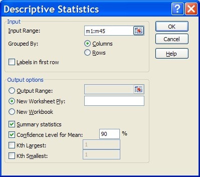
BE01106 Business Statistics Assignment image 10

In the Descriptive Statistics dialogue box you will need to tick the Confidence Level for Mean box and change the Confidence Level from the default 95% to the required 90% level.

The descriptive statistics table (with confidence interval estimation information included and the table modified to provide a more informative summary as described in Step 2 of Assignment Task 4) resulting from this process is:

Sold Price ($000)
Mean	551.211
Standard Error	34.573
Median	466
Mode	710
Std. Deviation	231.926
Sample Variance	53789.642
Kurtosis	-0.16
Skewness	0.46
Range	1068
Minimum	112
Maximum	1180
Maximum	1180
Sum	24804.5
Count	58.091

Note: The “Confidence Level(90.0%)” information, now provided in the descriptive statistics table, enables us to construct, in this instance, a 90% confidence interval estimate of the mean “Sold Price” of the population of properties. This value (58.091), for the data that forms the basis of this demonstration, has been rounded to three decimal places for consistency with the sample mean rounding as suggested in Step 2 of Assignment Task 4.

Step 2:

Deduce the point estimate and the 90% confidence interval estimate of the mean “Sold Price” of the population of properties from the sample “Mean” value and the “Confidence Level” information provided in the descriptive statistics table.

Remember that the “Mean” information provided in the descriptive statistics table is the mean of the sample data. You are required, in Assignment Task 6, to obtain two estimates, a point estimate and an interval estimate, of the mean “Sold Price” of the population of properties.

Further, note that the “Confidence Level” information, from the seminar material of week 7, is the value of “e” (error bound) that is subtracted and added to the sample mean to obtain the lower confidence limit (LCL) and upper confidence limit (UCL) respectively, of the appropriate confidence interval.

Step 3:

Copy the tabular output into a MS Word document to form part of your completed assignment.

Left click on cell A1 of the descriptive statistics table and then drag to highlight the entire contents of columns A and B. Then select the Copy icon from the Home menu and paste into your Word document as described in Step 3 of Assignment Task 4.

Assignment Task 7

In Task 7, you are required to use Excel to determine a point estimate and a 99% confidence interval estimate of the proportion of brick veneer properties in the population.

In order to achieve this we will need to obtain a descriptive statistics table, as per Assignment Task 6 above, but this time for a “new” set of sample data designed specifically to distinguish brick veneer from non-brick veneer properties (including vacant land) in your sample.

Step 1:

Transform the sample “Building Type” data (V4) into a “new” set of sample data designed specifically to distinguish brick veneer from non-brick veneer properties (including vacant land) in your sample.

Note that there are a number of techniques for doing this ranging from basic to the more sophisticated. The basic technique simply involves manually re-coding the values of variable V4 such that brick veneer properties are recorded as “1” and non-brick veneer properties (including vacant land) are recorded as “0”. A slightly more sophisticated technique might employ the use of the conditional “IF” function to achieve the same result.

The method employed in this demonstration will be the manual re-coding technique but feel free to use alternative methods if you so desire when completing the task for your data.

To make the manual process a little less tedious we will first sort the “Building Type” data (V4).

With your Excel workbook open at the sample data worksheet, click on cell E2 and then drag down to highlight the entire contents of column E, rows 2 to 51 (your sample “Building Type” (V4) data).

From the Home menu select the Copy icon and then paste the contents of cells E2 to E51 into any unused column, say, T1 to T50 (by activating cell T1 and then selecting the Paste icon).

With cells T1 to T50 highlighted, from the Data menu, Sort and Filter grouping, select the Sort Smallest to Largest (A to Z or Z to A) icon at which point the initial contents of cells T1 to T50 (your sample V4 values) will be sorted into ascending order.

Now, adjacent to the first “1” in column T (if there is one), type “0” in column U and press “Enter”. Immediately re-activate that cell and then moving the mouse cursor over the right hand bottom corner of it click on it when the cursor turns to a black cross and then drag vertically down column U until all the empty cells adjacent to cells with a “1” in column T have “0” copied into them.

Repeat this process for any cells in column U adjacent to cells in column T containing “3” or “4” in them at which point all non-brick veneer properties will be recorded in column U as “0”.

The “Building Type” data transformation is completed by following the process above for the first “2” appearing in column T but typing “1” in the adjacent empty cell in column U and then “clicking and dragging” to copy a “1” in all remaining empty cells of column U.

Data range U1:U50 will then contain values “0” and “1” only with the former representing non-brick veneer properties and the latter representing brick veneer properties.

Step 2:

Obtain a descriptive statistics table for the transformed “Building Type” sample data.

Repeat the procedure described in Step 1 of Assignment Task 7 above to obtain the descriptive statistics table suitable for constructing a point estimate and 99% confidence interval estimate for the proportion of brick veneer properties in the population.

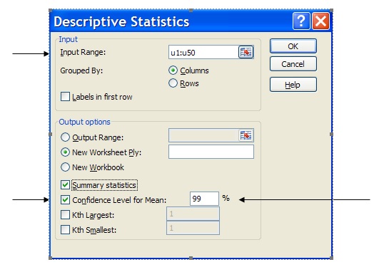
BE01106 Business Statistics Assignment image 11

In the Descriptive Statistics dialogue box you will need to specify, in the Input Range, the cell locations of the transformed sample “Building Type” variable i.e. u1:u50.

The Confidence Level for Mean box has been ticked and adjusted for 99% confidence.

The descriptive statistics table (with confidence interval estimation information included) resulting from this process is:

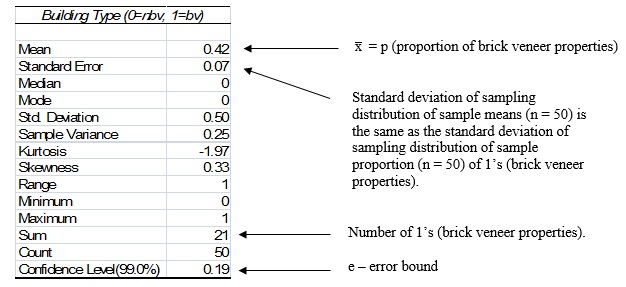
BE01106 Business Statistics Assignment image 12

Note: That the decimal values in this table have been rounded to, at most, two decimal places since the data being summarised in this table is whole number data (0’s and 1’s). This is consistent with the suggestion in Step 2 of Assignment Task 5.

At this stage you may be a little concerned that we have produced an Excel output that is going to provide information about a mean rather than a proportion.

The special feature to note here is that the transformed “Building Type” data consists entirely of 0’s and 1’s and because of this the “Sum” (in this case 21) actually represents the number of brick veneer properties (each represented by the number 1) in the sample of size fifty.

The “Mean” then, calculated as 21/50 = 0.42, as well as providing the arithmetic mean of the fifty data values (consisting of twenty-one 1’s and twenty-nine 0’s), also provides the percentage (21/50 = 42%) or proportion of brick veneer properties in the sample of size fifty.

Further, the “Standard Error” value of, in this case, 0.07, is, strictly speaking, the estimate of the standard deviation of the sampling distribution of sample means for samples of size fifty (in this case) used in the formula for constructing a confidence interval estimate of a population mean. Perhaps surprisingly, this “Standard Error” value, for a data set which consists entirely of 0’s and 1’s will be virtually identical (for large samples) to the standard deviation of the sampling distribution of sample proportions of 1’s for samples of size fifty (in this case) used in the formula for constructing a confidence interval estimate of a population proportion. This can be shown to be the case algebraically but is outside the scope of BEO1106.

Step 3:

Deduce the point estimate and the 99% confidence interval estimate of the proportion of brick veneer properties in the population from the sample “Mean” value and the “Confidence Level” information provided in the descriptive statistics table.

As explained above the “Mean” information provided in the descriptive statistics table for a data set consisting entirely of 0’s and 1’s also provides the proportion of 1’s in the sample data. You are required, in Assignment Task 7, to obtain two estimates, a point estimate and an interval estimate, of the proportion of brick veneer properties in the population.

Further, note that the “Confidence Level” information, from the seminar material of week 7, is the value of “e” (error bound) that is subtracted and added to the sample proportion to obtain the lower confidence limit (LCL) and upper confidence limit (UCL) respectively, of the appropriate confidence interval.

Step 4:

Copy the tabular output into a MS Word document to form part of your completed assignment.

Repeat the procedure described in Step 3 of Assignment Task 6 above.

Australia Universities

ACT

Australian Catholic University

Australian National University

Bond University

Central Queensland University

Charles Darwin University

Charles Sturt University

Curtin University of Technology

Deakin University

Edith Cowan University

Flinders University

Griffith University

Holmes Institute

James Cook University

La Trobe University

Macquarie University

Monash University

Murdoch University

Queensland University of Technology

RMIT University

Southern Cross University

Swinburne University of Technology

University of Adelaide

University of Ballarat

University of Canberra

University of Melbourne

University of Newcastle

University of New England

University of New South Wales

University of Notre Dame Australia

University of Queensland

University of South Australia

University of Southern Queensland

University of Sydney

University of Tasmania

University of Technology Sydney

University of the Sunshine Coast

University of Western Australia

University of Wollongong

Victoria University

Western Sydney University

Year 11 - 12 Certification Assignment

Australian Capital Territory Year 12 Certificate

HSC - Higher School Certificate

NTCE - Northern Territory Certificate of Education

QCE - Queensland Certificate of Education

SACE - South Australian Certificate of Education

TCE - Tasmanian Certificate of Education

VCE - Victorian Certificate of Education

WACE - Western Australia Certificate of Education

BE01106 Business Statistics Assignment

Assignment Part I

Assignment Part II

INSTRUCTIONS FOR OBTAINING EXCEL OUTPUTS FOR Tasks 2 - 4 OF THE BEO1106 ASSIGNMENT.

Tables, Graphs and Numerical Summaries of Data

INSTRUCTIONS FOR OBTAINING EXCEL OUTPUTS FOR TASKS 5 - 7 OF THE BEO1106 ASSIGNMENT.

Diploma Universities Assignments