Time Series Analysis: Linear Trend, Exponential Trend and Quadratic Trend

The data in Strategic represent the amount of oil, in billions of barrels, held in the U.S. strategic oil reserve, from 1981 through 2008.

A. Plot the data

Step 1: Copy the data and paste it into the Excel sheet.

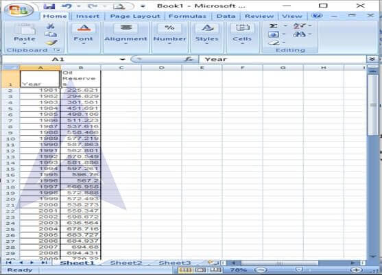
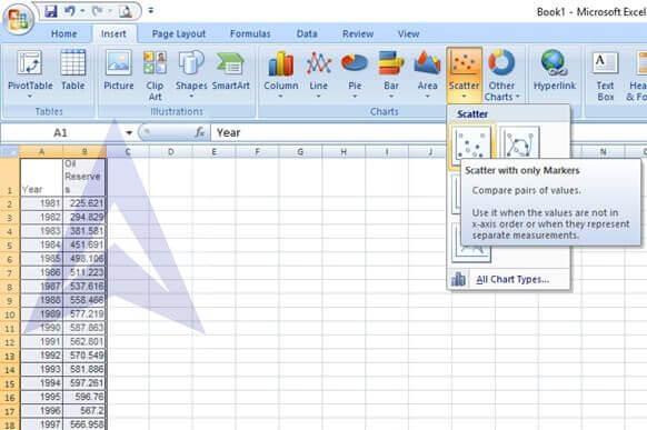
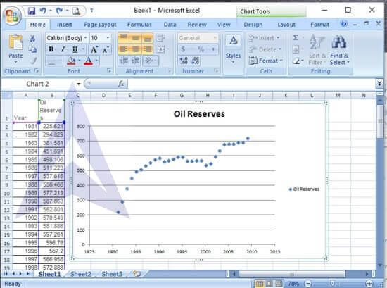
Step 2: To create a scatter plot of the data, go to Insert -> Scatter -> Scatter with only markers. The scatter plot will instantly display on the screen.

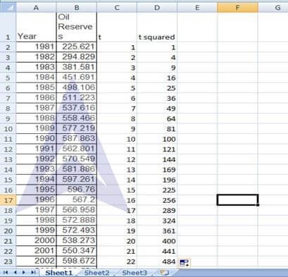
Assign a variable t depicting the years. Calculate the values of t squared corresponding to the t series.

{`
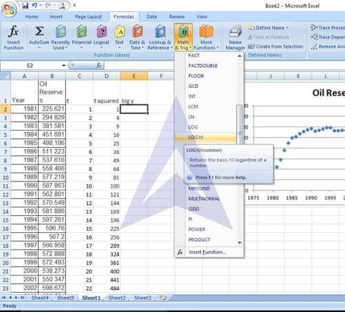
  Considering oil reserves as y, compute log y.
  Go to Formulas -> Math and Trigo -> LOG10
  In cell E2, enter the number as B2 under the LOG10 dialog box. Auto-fill this formula till cell E29.
  `}

B. Compute a linear trend forecasting equation and plot the trend line.

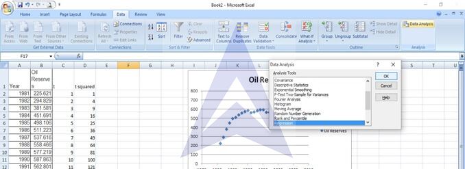
Step 1: To calculate the linear trend, go to Data -> Data Analysis.

Select the tool of Regression from the Data Analysis dialog box.

{`
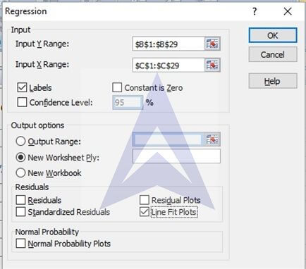
  Step 2: In the Regression dialog box, enter the following:
  Input y range: B1 to B29
  Input x range: C1 to C29
  Select the tick boxes: label, line fit plots.`}
  

Step 3: click on ok. The regression results are displayed:

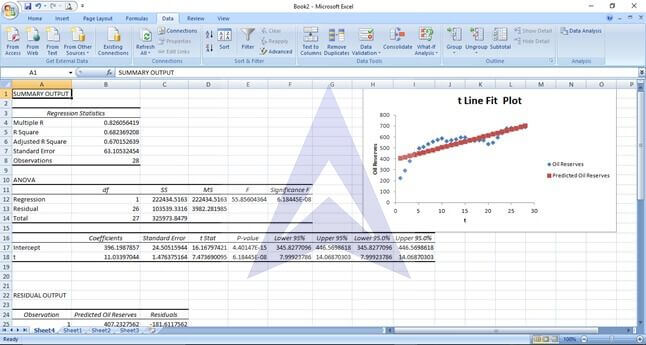
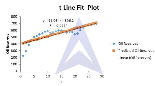
Step 4: From the regression coefficients given in the summary output, we get the following linear forecasting equation:

Y= 396.19 + 11.03 x
The plot of the trend line is:

C. Compute a quadratic trend forecasting equation and plot the results

Step 1: To calculate the quadratic trend, go to Data -> Data Analysis.
Select the tool of Regression from the Data Analysis dialog box.

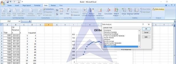
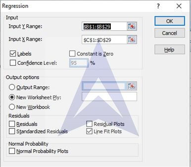
Step 2: In the Regression dialog box, enter the following:

{`
  Input y range: B1 to B29
  Input x range: C1 to C29
  Select the tick boxes: label, line fit plots.`}
  

Step 3: click on ok. The regression results are displayed:

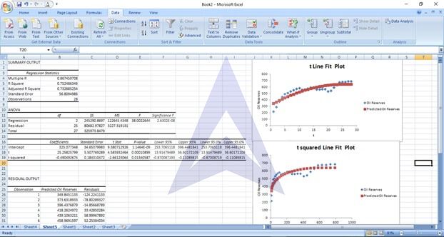
Step 4: From the regression coefficients given in the summary output, we get the following

linear forecasting equation:
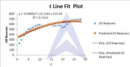
Y= 325.07 + 25.26 x -0.49 x2
The plot of the trend line is:

D. Compute an exponential trend forecasting equation and plot the results

Step 1: To calculate the exponential trend, go to Data -> Data Analysis.
Select the tool of Regression from the Data Analysis dialog box.

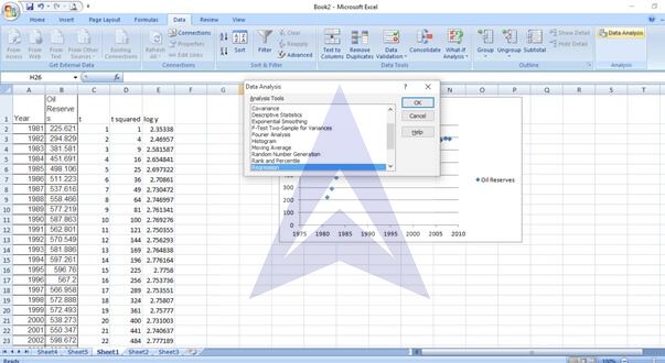
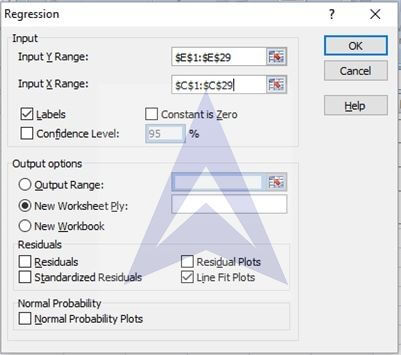
Step 2: In the Regression dialog box, enter the following:

Input y range: E1 to C29
Input x range: C1 to C29
Select the tick boxes: label, line fit plots.

Step 3: click on ok. The regression results are displayed:

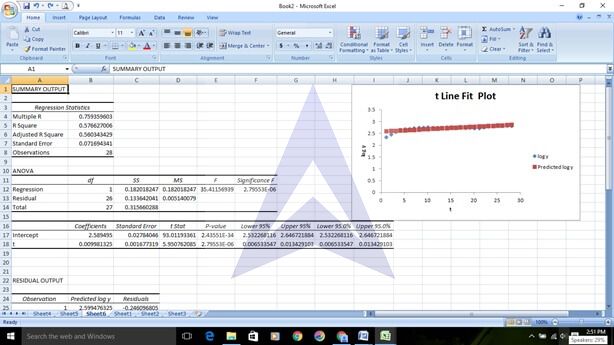
Step 4: compute the figure of 10^intercept.

{`
  The intercept comes out to be 388.59
  Now, we get the following exponential forecasting equation:
  Y = 388.59*10^0.0098*t
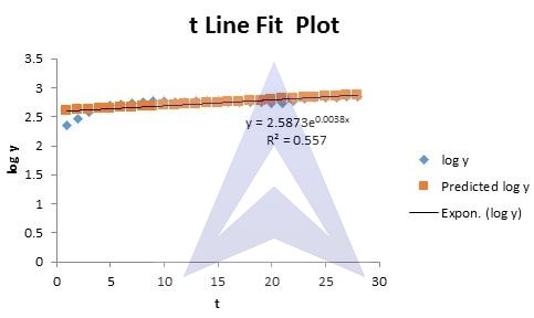
  Step 5: The plot of the trend line is:
  `}

E. Which model is the most appropriate?

The coefficients of determination for the three time series models we developed are:

{`
  Linear model_R2 = 68.24%
  Quadratic model_R2 = 75.25%
  Exponential_R2 = 55.7%
  `}

Since the coefficient of determination is the highest for the quadratic trend, therefore, the quadratic model seems the most appropriate

F. Using the most appropriate model, forecast the number of barrels, in billions, in 2009. Check how accurate your forecast is by locating the true value for 2009 on the Internet or in your library

• To predict the oil reserves in the year 2009, we take x = 29 and use the equation from the quadratic trend model. Y= -0.4905(29)² + 25.258(29) + 325.08 = 645.05 billions
• As per the exponential trendline, Y = 388.59*10^^0.0098*t, the prediction for oil reserves in the year 2009 (x = 29) will be 756.68 billions
• As per the linear trendline, Y= 396.19 + 11.03 x, the prediction for oil reserves in the year 2009 (x = 29) will be 716.18 Billions
• Actual value of the number of barrels, in billions, in 2009 = 720.22
• Based on this analysis, linear trend model seems to be the model of best fit with predicted values being closest to the observed values.

Excel Econometrics Tutorials

Multiple Regression Analysis

• Estimation and Inference
• Estimation, Inference & Prediction
• Model Formation: Checking Significance of Independent Variables

Time Series Analysis

• Exponential Smoothing Forecasting
• Plotting Linear Trend and Forecasting
• Monthly Data De-Trending, Seasonal Index & Forecasting
• Linear, Exponential and Quadratic Trend
• Excel Tutorial for Normal Distributions

Data Analysis

• Exploratory Data Analysis with Excel