Time Series Analysis: Exponential Smoothing Forecasting
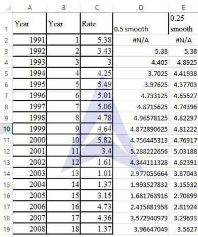
The following data (stored in Treasury) represent the three-month Treasury bill rates in the United States from 1991 to 2008:
| Year | Rate | Year | Rate |
|---|---|---|---|
| 1991 | 5.38 | 2000 | 5.82 |
| 1992 | 3.43 | 2001 | 3.40 |
| 1993 | 3.00 | 2002 | 1.61 |
| 1994 | 4.25 | 2003 | 1.01 |
| 1995 | 5.49 | 2004 | 1.37 |
| 1996 | 5.01 | 2005 | 3.15 |
| 1997 | 5.06 | 2006 | 4.73 |
| 1998 | 4.78 | 2007 | 4.36 |
| 1999 | 4.64 | 2008 | 1.37 |
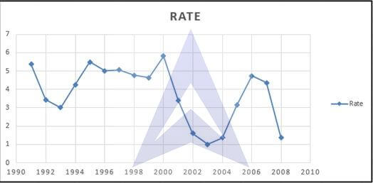
A. Plot the data
Step 1
Copy and paste data on excel
Step 2
Plot the line chart of the data by clicking on insert and click on the line chart icon. Select cells A1 to A19 for x axis values and cells B1 to B19 for y axis values.
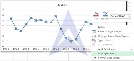
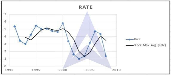
B. Fit a three-year moving average to the data and plot the results
Step 3
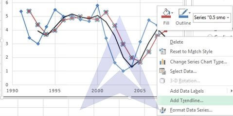
Select points the data points on the graph and right click. Click on the option add trend line. A dialogue box will appear select moving average and change the period to 3. Click ok.
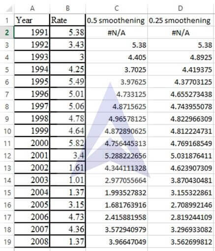
C. Using a smoothing coefficient of W = 0.50, exponentially smooth the series and plot the results
Step 4
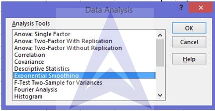
Click on data and select data analysis tool pack. A dialogue box opens. Select exponential smoothing from the dialogue box.
Step 5
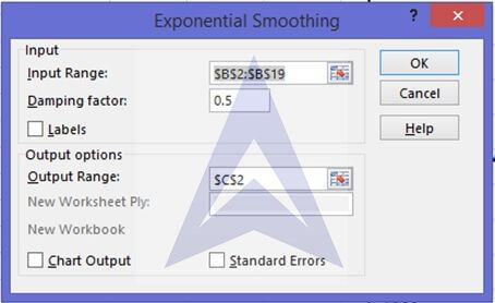
Select cells B2 to B19 as input range and enter the damping factor as 0.5 (damping factor= 1-smoothing factor (W)) and cell C2 as the starting cell for the output of the smoothing.
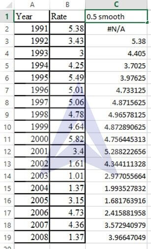
You will get the following data.
Step 6
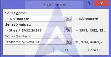
Right click on the graph. A dialogue box appears click on select data. And click on Add series.
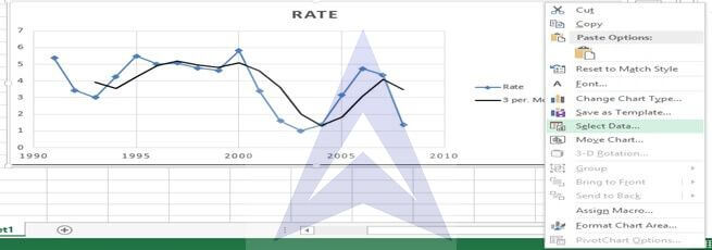
The following dialogue box appear. Name the series as 0.5 smooth and for x values select cells A2 to A19 and for y values select cells from C2 to C19. Click ok
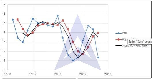
The following graphs appears
D. What is your exponentially smoothed forecast for 2009?
Step 7
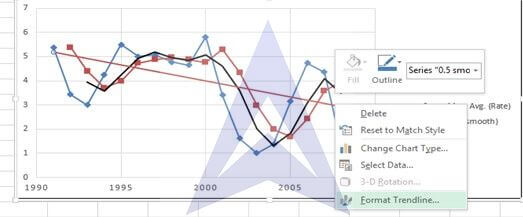
Click on the data points of the graph and right click. Select add trend line. A trend line will appear. Select the trend line and right click. Click on format trend line and select display equation andR2.
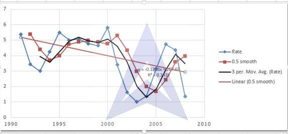
{`
  The forecast equation is
  Y= -0.1318*x + 5.3128
  For x=19 (2009)
  Y= -0.1318*19 + 5.3128
  = 2.8086
  `}
E. Repeat (c) and (d), using a smoothing coefficient of W = 0.25
Repeat steps 4-7. Take damping factor as 0.75
After completing the exponential smoothing steps as we did above the following output will be obtained
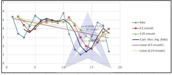
{`
  The exponentially smoothed Forecast equation when it is smoothed with W=0.25 is
  Y = -0.1285x + 5.5173
  The exponential smoothing forecast for 2009 is
  Y = -0.1285x + 5.5173
  = 3.0758
  `}
F. Compare the results of (d) and (e)
Comparing the results of D and E we can see that the results with exponential smoothing W=0.5 are closer to the actual data points. It can also be noted that the exponential smoothen trend with lesser W will have lesser peaks and valleys and will be farther from the actual data points when compared with exponential smoothened trend with higher W.
Excel Econometrics Tutorials
Multiple Regression Analysis
- Estimation and Inference
- Estimation, Inference & Prediction
- Model Formation: Checking Significance of Independent Variables
Time Series Analysis
- Exponential Smoothing Forecasting
- Plotting Linear Trend and Forecasting
- Monthly Data De-Trending, Seasonal Index & Forecasting
- Linear, Exponential and Quadratic Trend
- Excel Tutorial for Normal Distributions
Data Analysis


