Linear Regression Without Constant
n categories with n Dummy variables
When the explanatory variable is a dummy variable having n categories, we introduce only n-1 dummy variables. The coefficients of all such dummy variables is then interpreted as the difference between the corresponding dummy variable category compared to the base category. The impact of base category (for which no dummy variable is introduced) is represented by the constant intercept term. However, for n categories of dummy variable, we can also introduce n dummy variables. In this case, we run the regression without a constant term. Without dropping the constant term, there will be problem of autocorrelation. This method of running a dummy variable regression with no constant intercept term in STATA is outlined in this tutorial.
An alternative procedure for formulating the regression relationship in the previous question is as follows: First create a dummy variable called MA, defined as MA = 1 – FE (what does this variable denote?) Then estimate the following model: LNWAGE = γ1MA+ γ2FE + β1EDU + β2EX + β3EXSQ + ε
Interpret the estimates of γ1 and γ2 relating them to αM and αF above. According to economic theory, what would be the relationship among the estimates α1 and γ1, and α2 and γ2? Are your estimates consistent with this relationship? Formulate a test for the null hypothesis that there is no gender discrimination using the estimates of γ1 and γ2. What would be the problem of including an intercept in the model?
Creating a New variable in STATA
The command used for creating a new variable in STATA is
gen “new variable name” = ‘defining rule for new variable’
Thus in this example As instructed, we first create a dummy variable MA, defined as MA=1-FE as follows:
gen MA=1-FE
We then estimate the following model:
LNWAGE = γ1MA+ γ2FE + β1EDU + β2EX + β3EXSQ + ε
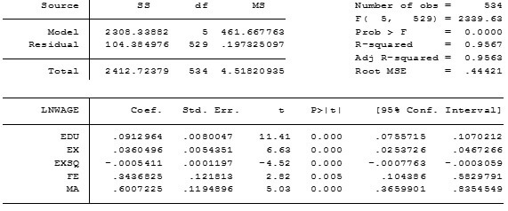
The regression output and the STATA command used for regression without constant term is given as follows:
regress LNWAGE EDU EX EXSQ FE MA, noconstant

Interpreting the STATA output of regression with no constant term
The value of coefficient γ1 is 0.6007225, which is interpreted as the minimum hourly wages in dollar (measured in logarithmic terms) that men (with no education and experience) receive in the given sample. The value of γ2 equals 0.3436 indicates the minimum hourly wage (measured in logarithmic terms) that female with no education and experience derives in the given sample. The γ1 equals α1 and γ2 equals α1 + α2. The relationship is apparent from the interpretations of these coefficients and estimates are consistent with the relationship.
Since this model and the model in previous part are the same, we use the finding in the previous part to conclude that is statistically significant gender discrimination in hourly wage earnings expressed in logarithmic terms.
When an intercept is added in the model, there will be a problem of autocorrelation as the constant term captures the same gender effect as MA component and MA variable will be omitted from the model owing to autocorrelation.
Checking for Difference in Returns using two sample T-test with equal variances in STATA
The specifications above take the returns to education to be constant for males and females. How would you test whether this assumption is correct? Perform the test.
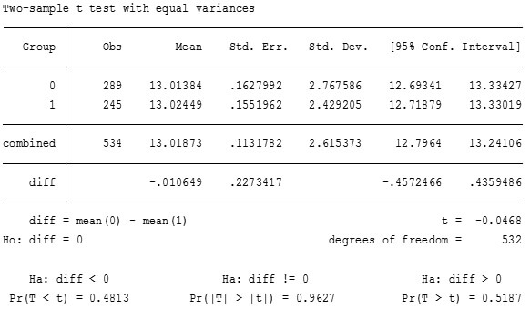
We test whether the return to education is constant for males and females using ttest in stata. The STATA command used for t-test and STATA test output obtained is
ttest EDU,by(FE)

Interpreting the STATA output for two sample t-test with equal variances
Based on the result obtained, we conclude that difference in returns to education for males and females is statistically insignificant at 5% level of significance. The reason is that value of t-statistic is less than 2 in absolute value and we therefore do not reject the null that there is no difference in returns to education for males and females. Also, p value is greater than 0.05, which implies statistical insignificance of the difference in returns to education at 5% level of significance.
Thus, the assumption that returns to education is constant for males and female is correct.


