Systems and signals square wave

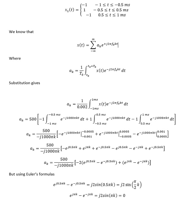
Case I: Square-wave x₁(t), 50% duty cycle

f₀=500 Hz

T_o=1/500=0.002s=2 ms

Mathematically, the square-wave can be expressed for a single period as

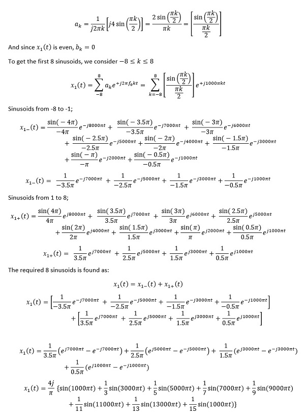
Therefore the trigonometric Fourier series coefficients of x₁(t) are

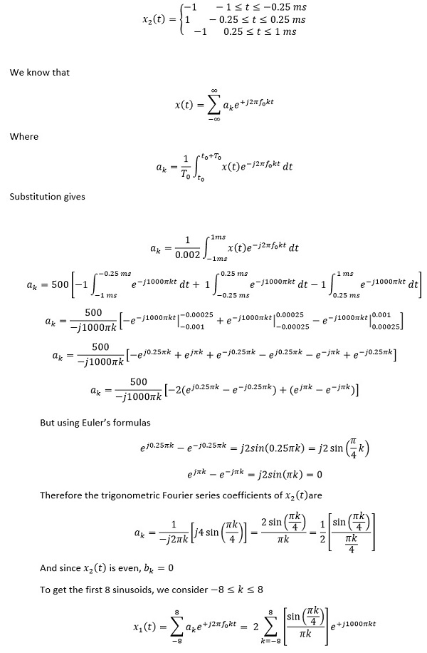
Case II: Square-wave x₂ (t), 25% duty cycle

Mathematically, the square-wave x₂ (t) can be expressed for a single period as

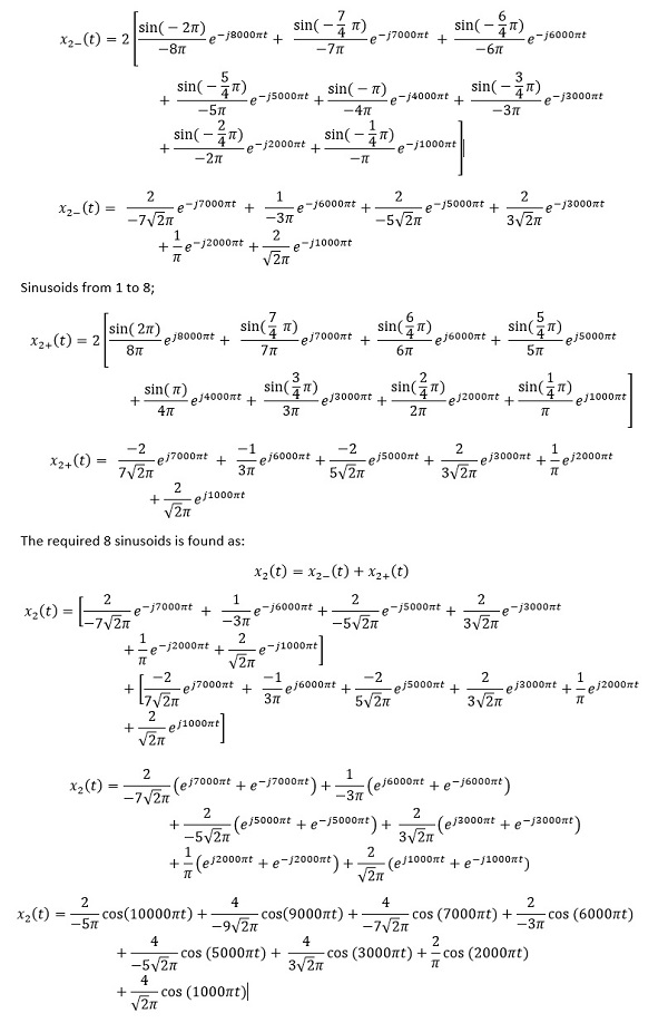
Sinusoids from -8 to -1;

{`
clear
clc
f_0= 500; % fundamental frequency
t= -0.001:0.00001:0.006; %time axis
Z_50= zeros(1,length(t)); % container for 50% duty cycle waveform
Z_25= zeros(1,length(t)); % container for 25% duty cycle waveform
n=1:16;
n1=sin(pi.*n./2);
d1=(pi.*n./2);
n2=sin(pi.*n./4);
d2=((pi).*n./4);
a_50=[n1./d1]; %fourier coefficients for 50% duty cycle
a_25=[0.5*(n2./d2)]; %fourier coefficients for % duty cycle
for k=1:length(n)
wa=1*cos(2*pi*(k)*f_0*t);
Z_50=Z_50+ a_50(k)*wa;
Z_25=Z_25+ a_25(k)*wa;
end
soundsc(Z_50)
figure (1)
plot(t,Z_50)
hold on
grid on
axis tight
xlabel('time')
ylabel('Amplitude')
title('Square-wave with 50% duty cycle');

figure(2)
plot(t,Z_25)
grid on
axis tight
xlabel('time')
ylabel('Amplitude');
title('Square-wave with 25% duty cycle');
`}