Design system for a pumped storage flow control system

1.1 Coursework Objectives

You have been engaged as a control engineering consultants to design system for a pumped storage flow control system. You will be expected to: work alone and will submit a formal report including the MATLAB code or SIMULINK.

• Derive the linear time invariant (LTI) differential equations for the system.
• Obtain the system’s response to a unit step input with and without initial conditions.
• Determine the state space model and the transfer function of the system.
• Analysis the system’s stability using MATLAB functions or SIMULINK.
• Design a state feedback controller to meet or exceed the response requirements.
• Obtain a discrete time model and design a state observer for the system.

• Submission:

The assignment submission should include: the report, a MATLAB script file (.m file) containing your calculation data (e.g. calculated gain values) and a SIMULINK file (.slx file) with your overall system (including controller implementation).

All calculations must be presented within the report. The report should include an introduction, results for each task, a discussion of findings, concluding statements and references. For each task, a proper description of the methodology is expected. For example, during block simplification, it is important to outline the process undertaken.

Report should be submitted for Similarity Check before submission to Google Classroom.

Page Limit 15 A4 Pages (single sided), with a minimum of 11 point font size. Appendices are not allowed.

Submission deadline: 11 September 2020

• Marking Scheme:

Coursework marks distribution is presented below. Refer to Marking Scheme (last page) for the overall mark scheme which will be used to grade discussion, introduction and conclusions components of the report, report presentation and referencing, and programs. Additional marks breakdown for calculations is provided in Section 2.

Report Marks Allocated

Derivation, analysis and calculations 90%

Report presentation, discussion and references 10%

Pumped Storage Flow Control System:

In this system, water is drawn off to supply a turbine to produce electrical power. The amount of water flow (Q_o), depends upon the fluctuating electrical power requirements of the turbine and generator. The water is supplied to the storage tanks from a secondary water supply. The two storage tanks are connected together through a shut-off valve, which may be modelled as a linear resistance R1. The resistance of the turbine supply pipe may be modelled as a linear resistance R2.

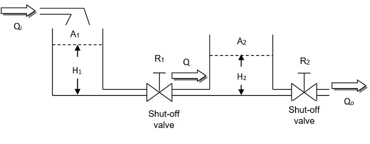
Figure 1

System Modelling

Given the following data to the system:

The cross sectional area of tank 1and tank 2 is 1 (m²). The linear resistance have the values R₁ = 0.5 s/m² and R₂ = 0.5 s/m²

Qo , Q_i ,Q = Volume flow rate (m³/sec)

A_1, A₂ = Cross sectional areas of the storage tank (m²)

R_1, R₂ = Proportionality constants of flow resistance (sec/m²)

H_1, H₂ = The height of the water level (m)

Q = (1/R)Δh ΔQ =A(Δh)

Problem 1 (10%)

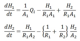
Show that the two tank system is described by the following set of differential equations.

Problem 2 (15%)

1. Using Laplace transforms obtain the responses of H_1, (t) and H₂ (t) when Q_i (t) is a unit step input and the initial conditions are H₁(0) = H₂ (0)= 0
2. Plot H_1, (t) and H₂ (t) of part (a) versus t and comment on the qualitative differences.
3. Obtain the plot H_1, (t) and H₂ (t) when Q_i (t)=0 and the initial conditions are H₁(0) = 10 and H₂ (0)= 0 comment on the qualitative differences.

Problem 3 (15%)

Open loop analysis

1. Obtain the state space representation for the system. [5 marks]

1. Determine the plant transfer function Q_o (s)/ Q_i (s). State the open loop poles and zeros. [10 marks]

Q_i (s)Q_o (s)

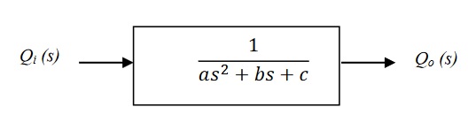
Figure 2 Open loop transfer function

Proportional control

Problem 4 –Stability analysis (15%)

Figure 3 shows proportional system with a unity feedback control loop. The demand flow (qd) would be set by a potentiometer having a unity gain. A variable gain K allows some adjustment to the system performance.

1. Find using the Routh array, the range of values of the gain K for the closed loop system to be stable.

[3 marks]

1. For the proportional controller gain K>0, plot the root locus diagram for the feedback control system of

Figure 3. [4 marks]

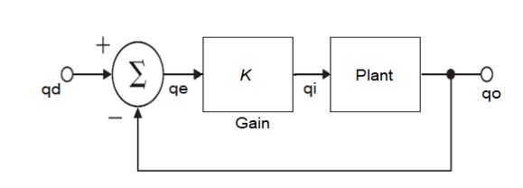
Figure 3

1. Determine the controller gain K;, for a unit step input the output response Qo (t) has a damping ratio of 0.8 and the maximum overshoot 1.48%. [8 marks]

Pole placement design

Problem 5 (20%)

1. Determine the controllability and observability of the plant. [5 marks]

2. Design a state feedback controller with the desired closed loop poles location at s = -5 + 2.23i,

s = -5- 2.23i. [10 marks]

1. Determine the closed loop transfer function. Simulate the closed loop response to a unitary step function input. [5 marks]

Discrete time system

Problem 6 (15%)

4. a) Obtain the discrete transfer function G(z) by taking the z-transform of G(s) when it connected as shown in Figure 4.

q_i(k) q_o(k)

T =0.1s

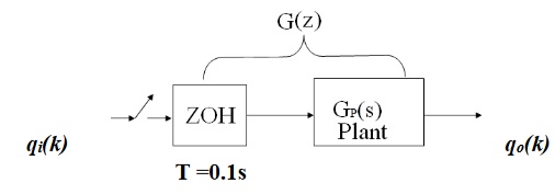
Figure 4

1. Find the state space representation in controllable canonical form for the discrete system.

15. Design a full order identity observer to place the desired observer poles at z = -15 and z = -15.

UFMFV7-15-2 (Control)

Mark sheet

Program/ Module: UFMFV7-15-2 (Control)

Assignment: Course Work