Measure of Central tendency Assignment Help
Exploratory Data Analysis
What is Data?
Data can be defined as any quantitative or qualitative values of a variable. Data involves facts and statistics collected together for analysis.
Sources of Data Collection
There are two sources of data collection:
a) PRIMARY SOURCES OF DATA:
The primary data refers to the original data that is collected by the researcher for the first time and for a specific purpose. Following are some of the sources through which primary data is collected:
- Questionnaire: A questionnaire contains a set of printed questions (multiple choice or subjective or both), devised for the purposes of survey or statistical study. Questionnaire can be done through telephonic call, e-mail etc.
- Survey: Survey refers to a brief interviews and discussions in order to draw specific information.
- Interviews: An interview is a face-to-face interaction with the respondent. It is a type of survey where a person asks load of in-depth questions from a person (respondent) in order to collect information about him/her.
Primary research done to collect primary data is a time consuming and expensive process.
b) SECONDARY SOURCES OF DATA:
Secondary data is that data which is collected by someone other than the user. It is that type of data that has already been collected and is readily available through different sources.
- Books- Books provide information on any topic of research and thus serve as an important source of secondary data. Books provides all the authentic information or knowledge required by the researcher to understand his subject on which he is working.
- Journals/periodicals- Journals and periodicals provide up-to-date information. Usually books provide data that are mostly on general topics of study. On the other hand, Journals provide research specific information and thus are important source of secondary data collection.
- Newspapers - Newspapers are very reliable source of secondary data collection. Newspapers provide a low cost and easily accessible information.
- Internet- Internet provides information on any subject matter that you are researching for. It is the fastest and inexpensive source of secondary data. Internet provides you the most recent and up to date information which is not possible with books or journals. Much information that is not available in printed form is available on the internet.
- Movies & documentaries may also serve some important information, helpful to anyone carrying secondary research in social sciences or humanities.
Random Sampling
Random sampling is a form of sampling technique in which each sample from a population has an equal probability of being chosen.
Measure of Central tendency Assignment Help By Online Tutoring and Guided Sessions from AssignmentHelp.Net
Following are different types of random sampling-
- SIMPLE RANDOM SAMPLING- In a simple random sample, each item of the population stands equal chance (probability) of being chosen.
- STRATIFIED RANDOM SAMPLING- this method involves division of the population into smaller groups known as strata. From each stratum, an item is selected randomly to form a random sample.
- CLUSTER SAMPLING- It is a sampling method in which the population is divided into different clusters. Then an item is drawn from each cluster randomly to form a random sample.
- SYSTEMATIC SAMPLING- this method of sampling requires a systematic rule to be followed in sample selection. Sampling data is collected on the basis of fixed interval. For example: From a data set of 10000 observations, every 3rd or 5th or 8th (any arbitrary number) must be included in the sample data
Population Census Versus Sample Survey
- A population census collects the information from all the participants of the population individually while sample survey uses the most representative group of participants in order to draw information about the whole population.
- In a population census, the whole universe is studied while in sampling survey, only a part of the universe is studied to draw results for the entire universe.
- Population census requires a lot of time, money and energy in order to collect data while sampling survey is less costly, and can be done in less time than taken by census.
- Population census is a reliable method of data collection. As the whole population is not studied in the sampling survey, the results drawn by it are less reliable.
- There is no scope of error in population census unless done properly. On the other hand, even if sampling survey is done properly without any bias, there is always some margin of error possible.
Univariate Frequency Distribution
In statistics, a frequency distribution is a tabular or graphical form that displays the frequencies of various outcomes in a sample.
In statistics, Univariate (“Uni” means “one” and “variate” means “variable”) is a commonly used term that describes a data which consists of observations on only a single attribute or characteristic (variable). In other words, a univariate distribution has only one variable.
Thus, when data is classified (summarized or grouped in the form of a frequency distribution) on the basis of a single variable, the distribution so formed is known as univariate frequency distribution.
Consider the following example of a univariate frequency distribution-
Following data shows the marks (variable) obtained in a test (out of100) by 60 students of a class-
Let the marks of students be denoted by variable X and number of students by f (frequency).
| Marks (X) | No. of students (f) |
|---|---|
| 20 | 12 |
| 30 | 8 |
| 40 | 10 |
| 50 | 20 |
| 60 | 4 |
| 70 | 6 |
| N=∑f=60 |
Measures of Central Tendency
Central tendency or an average is a middle or central point of a probability distribution.
According to Prof Bowley “Measures of central tendency (averages) are statistical constants which enable us to comprehend in a single effort the significance of the whole”.
Central tendency helps in summarizing the data in a single value and thus enabling comparisons between data.
Measures of central tendency or an average is a measure that attempts to describe a set of data with a single value that represents the middle or center of the distribution. Measure of central tendency includes:
- a) Locational or positional averages: this include partition values and mode. Partition values includes median, quartile, decile, and percentile.
- b) Mathematical averages: this include measures such as Arithmetic mean, Geometric mean and Harmonic mean.
Types of Averages
ARITHMETIC MEAN (OR MEAN)
Arithmetic mean (or simply mean or average) is the most commonly used method of representing the entire data set by one value. It is the most popular measure of central tendency as it is easily understandable.
Sample mean (X̅) refers to the mean of statistical samples while population mean (μ) is the mean of the whole population under study. Sample mean provides an estimate of the population mean. The formulae for calculating population mean and sample mean are same. Here, we analyze the concept of Arithmetic mean as a sample mean.
Arithmetic mean can be of two types:
- a) Simple arithmetic mean,
- b) Weighted arithmetic mean.
The mean is defined as the sum of numerical values of the observations in a data set divided by the total number of observations in that data set.
Sample mean or Arithmetic mean (here, we are analyzing Arithmetic mean as sample mean) is denoted by X̅.
SIMPLE ARITHMETIC MEAN
A. INDIVIDUAL SERIES
Direct method
Suppose we have a data set containing n observations with values b1, b2, b¬3, ……bn. In this case Arithmetic mean will be:
X̅= (b1+b2+b3+⋯+bn)/n
Or, X̅=∑b/n
Short cut method
Arithmetic mean in this method is calculated by using an arbitrary origin (A). this arbitrary origin is also known as assumed mean. The deviations of values are taken and then the following formula is used to find mean-
X̅=A+(∑d)/N
A=Assumed mean (arbitrary origin)
d= deviation of values from assumed mean=(X-A)
N=Number of observations
Arithmetic mean in case of ungrouped Frequency distribution
Direct method
Formula for mean calculation under direct method is as follows-
X̅=∑fX/N
f= Frequency
X= the value of variable in question
N=∑f= Total no of observations
Short-cut method
The formula used in this method is-
X̅=A+∑fd/N
A=Assumed mean (arbitrary origin)
d=(X-A)
N=∑f= Total no of observations
B. CONTINUOUS SERIES (grouped frequency distribution)
Grouped frequency distribution is the organizing of the raw data using classes and frequencies.
In a continuous series, instead of individual values like 10, 20, 30, …n, we have data in the form of class intervals such as 10-20, 20-30, 30-40….so on.
Direct method
Under this method the following formula is used to calculate the mean-
X̅=∑fm/N
m= mid-point of various classes given in question
f= frequency of each class
N=∑f= Total no of observations
Short-cut method
This method suggests the use of following formula to calculate arithmetic mean-
X̅=A+(∑fd)/N
A=Assumed mean (arbitrary origin)
d=(m-A) = deviation of mid-points from assumed mean
N=∑f= Total no of observations
Step Deviation method
Following formula is used under this method- X̅=A+(∑fd)/N×h
A=Assumed mean (arbitrary origin)
d=(m-A) = deviation of mid-points from assumed mean
N=∑f= Total no of observations
h = Class interval (example- when we have a class 30-40, the class interval here is 10)
Properties of Arithmetic mean
- The sum of deviations of items in a data set from the arithmetic mean is always 0 i.e. ∑(X-X̅ ) = 0. {∑f(X-X̅) = 0 in case of frequency distribution}
- The sum of squared deviations of the items from the arithmetic mean is always minimum i.e. ∑(X-X̅)2 = minimum.
- Arithmetic mean is capable of further mathematical manipulations. If we are given the arithmetic means and number of items of two or more than two related groups, then it is possible to combined average of these groups by applying the formula given below-
X̅1̅2̅ = N1X̅1̅+N2X̅2̅ / N1+N2
X̅1̅2̅ = Combined mean of the two groups
X̅1̅ = Arithmetic mean of the 1st group
X̅2̅ = Arithmetic mean of the 2nd group
N1 = no of items in the 1st group
N2 = No of items in the 2st group - If we have two variables X and Y and the observations of both the variables are linearly related as
Y = a + bX, then
Y̅ = a + bX̅
Weighted Arithmetic Mean
Simple arithmetic mean gives equal importance to all the items in a data set. However, there may be some items whose relative importance in the data is not same. The weighted arithmetic mean helps in calculation of mean by assigning weights to each item. The term weight here stands for the relative importance of different items of the data.
The formula required to calculate arithmetic mean is as follows-
X̅w = ∑WX/∑W (individual series)
X̅w = ∑W(fX)/∑W (frequency distribution)
Advantages of Arithmetic mean
- Arithmetic Mean is rigidly defined
- Arithmetic Mean is easy to understand
- Arithmetic Mean is based on each and every item of the distribution.
- Arithmetic Mean is capable of mathematical manipulation such as change of scale and change of origin.
Disadvantages and Problems of Arithmetic mean
- Arithmetic Mean gets affected by extreme values (outliers).
- Arithmetic Mean cannot be calculated for data having open-ended classes.
- Arithmetic Mean cannot be located graphically.
Geometric Mean
Geometric mean is defined as the nth rood of the product of N items or values.
GM = n√(X1)×(X2)…×(Xn))
Where X1, X2, X3 etc. represent various items of the series.
- In case of individual series, we use the following formula- GM = antilog( ∑logX)/ N )
- In case of ungrouped frequency distribution, we have items X1, X2, X3…. Xn and corresponding frequencies as f1, f2, f3…… fn. The formula used to calculate Geometric mean is- GM = antilog( ∑flogX)/ N )
- In case of grouped frequency distribution, we use the following formula- GM = antilog(∑flog(m)) / N )
Where m = midpoint of various classes given in question
Merits of Geometric mean
- Geometric Mean is based on each and every item.
- Geometric Mean is rigidly defined
- Geometric Mean is capable of mathematical manipulations.
Demerits of Geometric mean
- The concept of Geometric mean can be difficult to understand.
- Geometric mean is difficult to compute and interpret.
- Geometric Mean is affected by extreme values.
- Geometric Mean cannot be located graphically.
HARMONIC MEAN
Harmonic mean is defined as the reciprocal of the arithmetic mean of the reciprocal of the individual observation.
HM = N /(1/X1 + 1/X2 + ⋯ + 1/Xn)
In individual series, HM = N / ∑(1/X)
In ungrouped frequency distribution, HM = N / ∑(f×1/X)
In grouped frequency distribution, HM = N / ∑(f×1/m)
Where m = mid-point of various classes given in question
Merits of Harmonic mean
- Rigidly defined.
- Based on each and every item of the distribution.
- Capable of mathematical manipulations.
Demerits of Harmonic mean
- Difficult to compute.
- Affected by extreme values.
- Cannot be located graphically.
- Cannot be calculated in case of open-ended classes
Mode
Mode or the modal value is that value in a series of observations which has the highest frequency. For example, the mode of the individual series 3,5,7,5,6 would be 5 as this value occurs more frequently than any other value in the series.
There may be no unique modal value in a series. There may be two modes (known as bimodal), three modes (known as tri modal). When there are more than three modes, it will be a case of multi modal.
- In case of ungrouped frequency distribution, the item with maximum frequency represents the mode.
- When we have grouped frequency distribution, then first we need to calculate the modal class in which the modal value lies. The modal class is that class which has the largest frequency. After we have identified the modal class, then we use the following formula to calculate the modal value of the distribution. We use the following formula-
Mode = L + (f1-f)/(2f1-f0-f2) × h
Where L= Lower limit of the modal class
f1 = frequency of the modal class
f0 = frequency of the class preceding the modal class
f2 = frequency of the class succeeding the modal class
h = class interval of the modal class
- The above formula can be used only when the class intervals are uniform throughout the distribution.
- The above formula cannot be used when we are given a multimodal distribution. In this case we calculate empirical mode using the following relation- Mode = 3 Median-2 Mean
Merits of Mode
- Mode is the most representative value of any distribution.
- Mode is not affected by outliers (extreme items).
- Mode can be used in open-end distributions without knowing the class limits.
- Mode is possible to locate graphically.
- Mode is easy to understand, interpret and calculate.
Demerits of mode
- Mode is not rigidly defined.
- Mode is not capable of mathematical manipulations
- The Value of mode is not based on each and every item of the series.
Median
Median refers to the middlemost value in a distribution. It is known as a positional average. A change in the value of a single item will not cause any change in the value that divides the observations into two equal parts.
- In order to find median, the data must be first ranked in ascending or descending order.
- In case of individual series, when there are odd number of observations, median is the middle value (= size of (N+1)/2 th item). However, when the data contains even number of observations, then the median is the mean of the two middle values.
Calculating Median of Ungrouped Frequency Distribution
Cumulative frequency in simple words refers to the running total of all the frequencies.
Consider an Example-
| X (income) | No. of person (f) |
|---|---|
| 200 | 24 |
| 250 | 26 |
| 180 | 16 |
| 300 | 20 |
| 350 | 6 |
| 280 | 30 |
Solution-
In order to find median, we first rank the income in ascending order and then calculate cumulative frequency.
| X (income) | No. of person (f) | Cumulative frequency (cf) |
|---|---|---|
| 180 | 16 | 16 |
| 200 | 24 | 40 |
| 250 | 26 | 66 |
| 280 | 30 | 96 |
| 300 | 20 | 116 |
| 350 | 6 | 122 |
N=122
Median = size of (N+1)/2 th item
Median = 122+1/2 th item
Therefore, Median = 61.5th item
From the cumulative frequency column, we find that
61.5th item = 250.
Hence, Median = 250
Calculating Median of Grouped Frequency Distribution
- In grouped frequency distribution, we are given different classes. So first we have to find that particular class in which the value of median lies.
The formula used to find median after we have the median class is-
Median = L + (N/2-cf/ f) × h
Where L= Lower limit of the median class
cf= Cumulative frequency of the class preceding the median class
f= Frequency of the median class
h= Class interval of the median class
In case of grouped frequency distribution, we use N/2 as the rank of the median instead of (N+1)/2.
Dispersion
According to Spiegel “The degree to which the numerical data tend to spread about an average value is called the dispersion of the data”.
Dispersion measures the extent to which the items vary from some central value.
Measuring Dispersion (variation)
- - It is necessary to measure the amount of variation in the data from the central value in order to determine the reliability of the average and to compare two or more series with regard to their variability.
- - Measures of dispersion may be either absolute or relative. Absolute measures are expressed in same statistical unit as the original data are given. On the other hand, relative dispersion is used when two or more set of data are defined in different units.
Range
Range is the simplest method of studying dispersion. It is defined as the difference between the value of the smallest item and the value of the largest item included in the distribution.
Range = Largest value – smallest value
Relative measure of range is known as coefficient of range.
Coefficient of range = (L-S)/(L+S)
Where L= Largest value
S= smallest value
Merits of Range
- Simplest to understand and easy to calculate.
- Gives rough idea about the variation in the data quickly.
Demerits of Range
- Not based on each and every item.
- Subject to fluctuations from sample to sample.
- Unreliable and inaccurate guide of dispersion.
Quartile Deviation
Quartile deviation or semi-interquartile range includes the middle 50% of the distribution only. Interquartile range refers to the difference between the third quartile (Q3) and first quartile (Q1).
Interquartile range = Q3 - Q1
Quartile deviation (QD) is represented as-
QD = (Q3 - Q1)/2
Quartile deviation gives the average amount by which the two quartiles differ from the median. Coefficient of quartile deviation which is a relative measure is calculated as follows-
QD = (Q3 - Q1)/(Q3+ Q1)
This relative measure is used to compare the degree of variation in different distributions.
Merits of Quartile deviation
- Quartile Deviation is superior to range as a measure of dispersion.
- Quartile Deviation is not affected by the presence of extreme values.
Demerits of Quartile deviation
- Quartile Deviation is not based on each and every item.
- Quartile Deviation is Not capable of mathematical manipulations.
- Quartile Deviation is affected by sampling fluctuations.
Mean Deviation
Mean deviation is the average difference between the items (X) in a distribution from mean or median of that series of data.
MD or mean deviation = (∑∣D∣)/N (In individual series)
Where, ∣D∣ is the absolute value of the deviation from median or mean.
MD or mean deviation = (∑f∣D∣)/N (In ungrouped frequency distribution)
∣D∣ = ∣X-Me/mean∣
MD or mean deviation = (∑f∣D∣)/N × h (In grouped frequency distribution)
∣D∣ = ∣m-median/mean∣
(m=midpoint of classes in question)
- Relative measure for mean deviation is given as, Coefficient of MD = MD/Mean or MD/Median
Merits of Mean deviation
- Easy to understand and compute.
- Based on each and every item of the data.
- Less affected by extreme values as compared to standard deviation.
Demerits of Mean deviation
- While taking the deviations, algebraic signs of values are ignored.
- Does not give accurate results.
- Not capable of mathematical manipulations.
Standard Deviation
Standard deviation is also known as root mean square deviation and measures the absolute dispersion or variation of a distribution. Higher standard deviation implies high degree of variability.
Calculating Standard Deviation
Following formulae are used to calculate standard deviation for different distributions-
When deviations are taken from Actual mean (X̅)
Individual series - SD = √((∑x∧2)/N) where x = (X-X̅)
Ungrouped frequency distribution- SD = √((∑f(x∧2))/N) where x = (X-X̅)
grouped frequency distribution- SD=√(∑f(x∧2)/N) where x = (m-X̅) {m is the midpoint of classes in question}
When deviations are taken from Assumed mean (A)
Individual series- SD = √((∑d∧2)/N-((∑d)/N)∧2) where d = (X-A)
Ungrouped frequency distribution- SD=√(∑f(d∧2)/N-((∑fd)/N)∧2) where d = (X-A)
grouped frequency distribution- SD=√(∑f(d∧2)/N-((∑fd)/N)∧2) ×h where d = (X-A)/h
and h = class interval
Merits of Standard deviation
- Based on every item of the distribution.
- Capable of mathematical manipulations (possible to compute combined SD).
- Less affected by sampling fluctuations.
Demerits of Standard deviation
1. Difficult to compute compared to other measures of dispersion.
SKEWNESS AND KURTOSIS
Skewness
Skewness refers to the asymmetry or lack of symmetry in the shape of a frequency distribution. In other words, when a distribution is not in symmetry, it is called a skewed distribution.
A distribution may be positively skewed or negatively skewed.
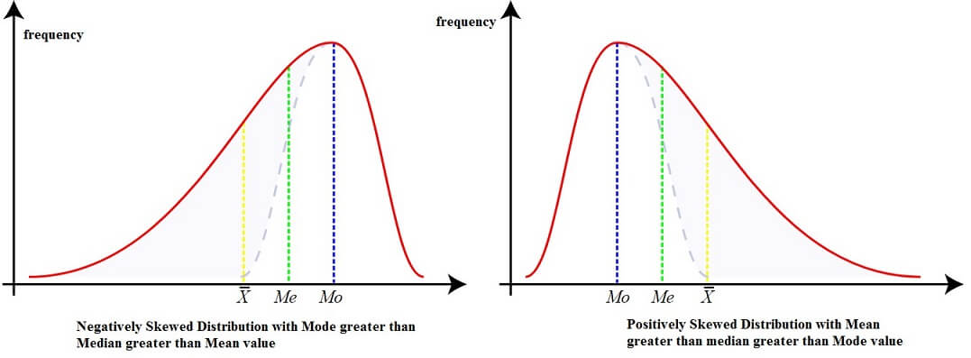
- When the distribution is positively skewed, then the frequencies (Y-axis) in the distribution are spread out over a greater range of values (on X-Axis) on the high-value end of the curve (right hand side).
When the distribution is negatively skewed, then the frequencies (Y-axis) in the distribution are spread out over a greater range of values (X-axis) on the lower-value end of the curve (left hand side).
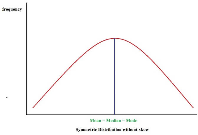
Positively skewed Distribution or Skewed towards right whereas a Negatively skewed distribution or skewed to Left. When the curve is normally spread, frequencies will be symmetric and equally distributed on both the sides of the mid-point (or center point) and the mean, median and mode will all be equal. A or symmetrical distribution is shown as follows:
Statistical analysis is most often based on the concept of a bell-shaped symmetrically distributed normal distribution.
In a positively skewed distribution or a distribution that is skewed to the right, the value of mean (X̅) is maximum and value of mode (Mo) is the least. Median (Me) lies in the middle of the two. { X̅> Me > Mo}
In a negatively skewed distribution or a distribution that is skewed to the left, the value of mode (Mo) is maximum, the value of mean (X̅) is the least and Median (Me) lies in the middle of the two. { X̅< Me < Mo}
In a symmetric distribution, the value of mean is equal to the value of mode and is equal to the value of median
Measures of skewness
Measures of skewness helps in accessing the direction as well as the degree of asymmetry in a given data set. These measures can be absolute as well as relative.
Absolute measures of skewness
The difference between the mean (X̅) and mode (Mo). If the value of the mean is greater than the mode, then the skewness will be positive (+). Conversely, if the value of mean is less than the value of Mode, then the skewness will be negative (-).
Absolute Sk = X̅ - Mo
Absolute skewness can also be expressed in terms of quartiles:
Absolute Sk = Q1+Q3-2Me
Relative measures of skewness
Relative skewness involves three measures:
1. The Karl Pearson’s coefficient of Skewness (SKp): This relative measure of skewness is based upon the Absolute measure of skewness which is the difference between mean and mode. when this difference is divided by standard deviation, we get a relative measure. The formula is as follows:
SKp = (Mean-Mode)/(Standard deviation)
The above formula of relative skewness gives direction as well as the degree of skewness. However, the formula cannot be used when a distribution is bimodal. In this case we use the following relation between mean, median and mode-
Mode=3Median-2Mean
Using the above relation, we get the following formula for calculating relative skewness-
SKp=(3(Mean-Median))/(Standard deviation)
2. Bowley’s coefficient of skewness (SKb): This measure is based on the concept of quartiles. In a normal or symmetrical distribution, the 1st and the 3rd quartiles are equidistant from the 2nd quantile i.e. the median-
Q3+Q1-2Median=0
The formula for Bowley’s coefficient of skewness is given as-
SKb = (Q1+Q3-2Median)/(Q3-Q1)
Bowley’s measure of skewness is based on the middle 50% of the observations in a data set. The skewness analysis here leaves the top 25% and lowest 25% of the observations.
3. Kelly’s coefficient of Skewness (SKk): Skewness is concerned with the extreme values in a data. Clearly, Bowley’s measure of relative skewness does not include the extreme values. Kelly’s measure of relative skewness is based on 10th and 90th percentile (or 1st and 9th decile). The formula for Kelly’s coefficient of skewness can be shown as follows-
SKk = (P10+P90-2Median)/(P90-P10)
Kurtosis
What is Kurtosis?
In statistical theory, Kurtosis is a measure of extent of flatness or tailedness in a frequency distribution curve.
Kurtosis of a distribution curve is usually studied relative to a normal (symmetric) distribution curve.
A curve, depending on the degree of flatness, can be mesokurtic (normal distribution curve), leptokurtic or platykurtic.
MESOKURTIC
A distribution is said to be Mesokurtic when the kurtosis of that distribution is same as the kurtosis of the normal distribution. Kurtosis of a univariate normal distribution is 3.
LEPTOKURTIC
A distribution which has positive excess kurtosis (kurtosis greater than 3). This type of distribution has a curve that is more peaked than the normal distribution curve.
PLATYKURTIC
A distribution which has negative excess kurtosis (kurtosis less than 3). This type of distribution has a curve that is less peaked or say, is flatter than the normal distribution curve.
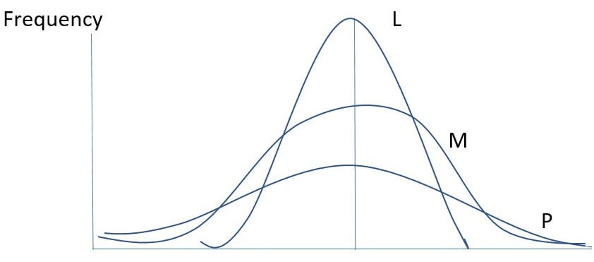
L-LEPTOKURTIC
M-MESOKURTIC
P-PLATYKURTIC
The above diagrammatical description of different regimes of Kurtosis (L, M, P) makes it clear that they differ widely with respect to convexity.

Best Online Statistics Homework Help Tutors
At assignmenthelp we have the best statistics tutors for online homework help with statistics assignments, business statistics essay research writing as well as for statistical analysis related custom research writing work. Our statistics Assignment Help tutors are well versed in techniques of data analysis including exploratory data analysis as well as advanced statistical analysis techniques of regression, ANOVA, F test, T test, Chi-square test, time series analysis, multiple regression analysis and more. Advanced statistical analysis such as Panel data regression and time series modelling are useful not just for statistics students but also for students studying econometrics, finance, psychology, research methods, biology, medical science and social sciences etc. At Assignment Help we also provide free statistical analysis tutorials on software like STATA, SPSS, Excel, R and many more.


