When follow connection from the current node

Chapter 4 Pathfinding
Start	1	1	1	1	1	1
1	1	1	1	1	1	1
1	1	1	1	1	1
1	1	1	1	1	1

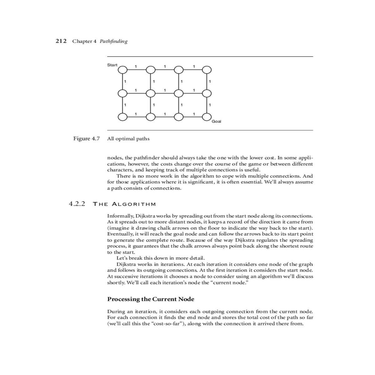
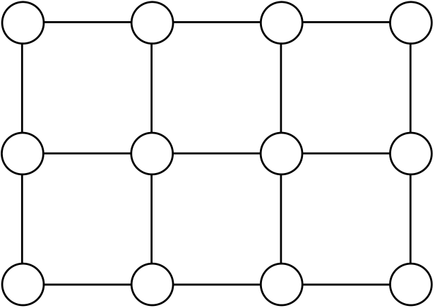
Figure 4.7	All optimal paths

4.2.2 THE ALGORITHM

Informally, Dijkstra works by spreading out from the start node along its connections. As it spreads out to more distant nodes, it keeps a record of the direction it came from (imagine it drawing chalk arrows on the floor to indicate the way back to the start). Eventually, it will reach the goal node and can follow the arrows back to its start point to generate the complete route. Because of the way Dijkstra regulates the spreading process, it guarantees that the chalk arrows always point back along the shortest route to the start.

4.2 Dijkstra 213

current		B
current	cost: 1.3	B	connection: I

	Connection II
	cost: 1.6
Connection III	C
Connection III	C	connection: II

cost: 3.3

	D
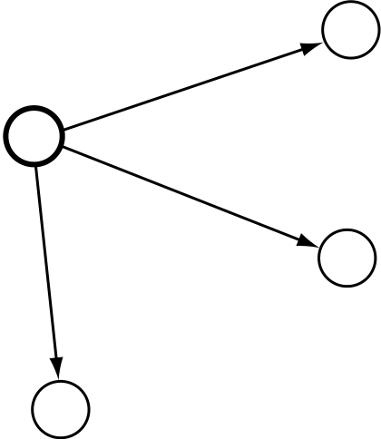
Figure 4.8	Dijkstra at the first node
	current						E
	current						E
	start	Connection I		node	B	Connection IV		cost-so-far: 3.2
		Connection I				cost: 1.5
		cost: 1.3
	node	cost: 1.3
	cost-so-far: 0		Connection II			Connection V	F
			cost: 1.6			Connection V
			cost: 1.6			cost: 1.9
	Connection III		C
	Connection III		C			connection: II
	cost: 3.3
	D
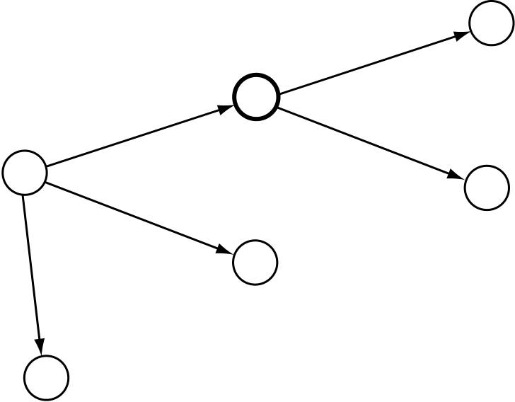
Figure 4.9	Dijkstra with a couple of nodes

The Node Lists

The algorithm keeps track of all the nodes it has seen so far in two lists, called “open”and “closed.” In the open list it records all the nodes it has seen, but that haven’t had their own iteration yet. It also keeps track of those nodes that have been processed in the closed list. To start with, the open list contains only the start node (with zero cost-so-far), and the closed list is empty.

If we arrive at an open or closed node during an iteration, then the node will already have a cost-so-far value and a record of the connection that led there. Simply setting these values will overwrite the previous work the algorithm has done.

Instead, we check if the route we’ve now found is better than the route that we’ve already found. Calculate the cost-so-far value as normal, and if it is higher than the recorded value (and it will be higher in almost all cases), then don’t update the node at all and don’t change what list it is on.

						E	4.2 Dijkstra
							cost-so-far: 2.8
							connection: IV
start					Connection IV
					cost: 1.5

node
cost-so-far: 0	A	Connection II		Connection V		F
connection: none		cost: 1.6		Connection V			connection: V
connection: none		cost: 1.6		cost: 1.9
Connection III		Connection VI			cost-so-far: 1.6 connection: II
Connection III			current
cost: 3.3			current
node

		Is updated	cost-so-far: 2.9	Open list	Closed list
	connection: III		connection: VI	E, F, D
Figure 4.10	Open node update

The basic Dijkstra algorithm terminates when the open list is empty: it has considered every node in the graph that be reached from the start node, and they are all on the closed list.

For pathfinding, we are only interested in reaching the goal node, however, so we can stop earlier. The algorithm should terminate when the goal node is the smallest node on the open list.

Chapter 4 Pathfinding							cost-so-far: 2.8
						E	cost-so-far: 2.8
						E
start					Connection IV		cost-so-far: 3.2
					cost: 1.5

node
cost-so-far: 0	A	Connection II	Connection V			F
connection: none		cost: 1.6	Connection V
			cost: 1.9
			cost: 1.9
Connection III			C	cost-so-far: 1.6
				connection: II

cost: 3.3
D			goal				G	cost-so-far: 4.6
cost-so-far: 2.9			node

Connections working back from goal: VII, V, I Final path: I, V, VII

Figure 4.11	Following the connections to get a plan

longer. For this reason, many developers implement their pathfinding algorithms to terminate as soon as the goal node is seen, rather than waiting for it to be selected from the open list.

4.2.3 PSEUDO-CODE

The Dijkstra pathfinder takes as input a graph (conforming to the interface given in the previous section), a start node, and an end node. It returns an array of connection objects that represent a path from the start node to the end node.