

Was supported partly dfg-snf lead agency program grant grant
KLOOSTERMAN PATHS AND THE SHAPE OF EXPONENTIAL SUMS
EMMANUEL KOWALSKI AND WILLIAM F. SAWIN
the normalized classical Kloosterman sum, where ψp(z) = e(z/p) = e2iπz/pis the standard |
|---|
| 1⩽x⩽j+1� |
|
|
|---|---|---|
|
||
1
0.1
| � 1.5 | � 1.0 | � 0.5 |
|---|
� 0.1
We will use the computation of monodromy groups of Kloosterman sheaves to find the
limiting distribution of (Kp(t)) as p → +∞, in the sense of convergence of finite distributions.
converges almost surely and in law, taking symmetric partial sums, where the term h = 0 |
|---|
is interpreted as tST0. Its limit, as a random function, is almost surely continuous. In
· · · < tk ⩽ 1, the vectors
(Kp(t1), . . . , Kp(tk))
| converge in law, as p → +∞, to |
|---|
0.3
0.2
| � 0.2 | 0.2 | 0.4 |
|---|
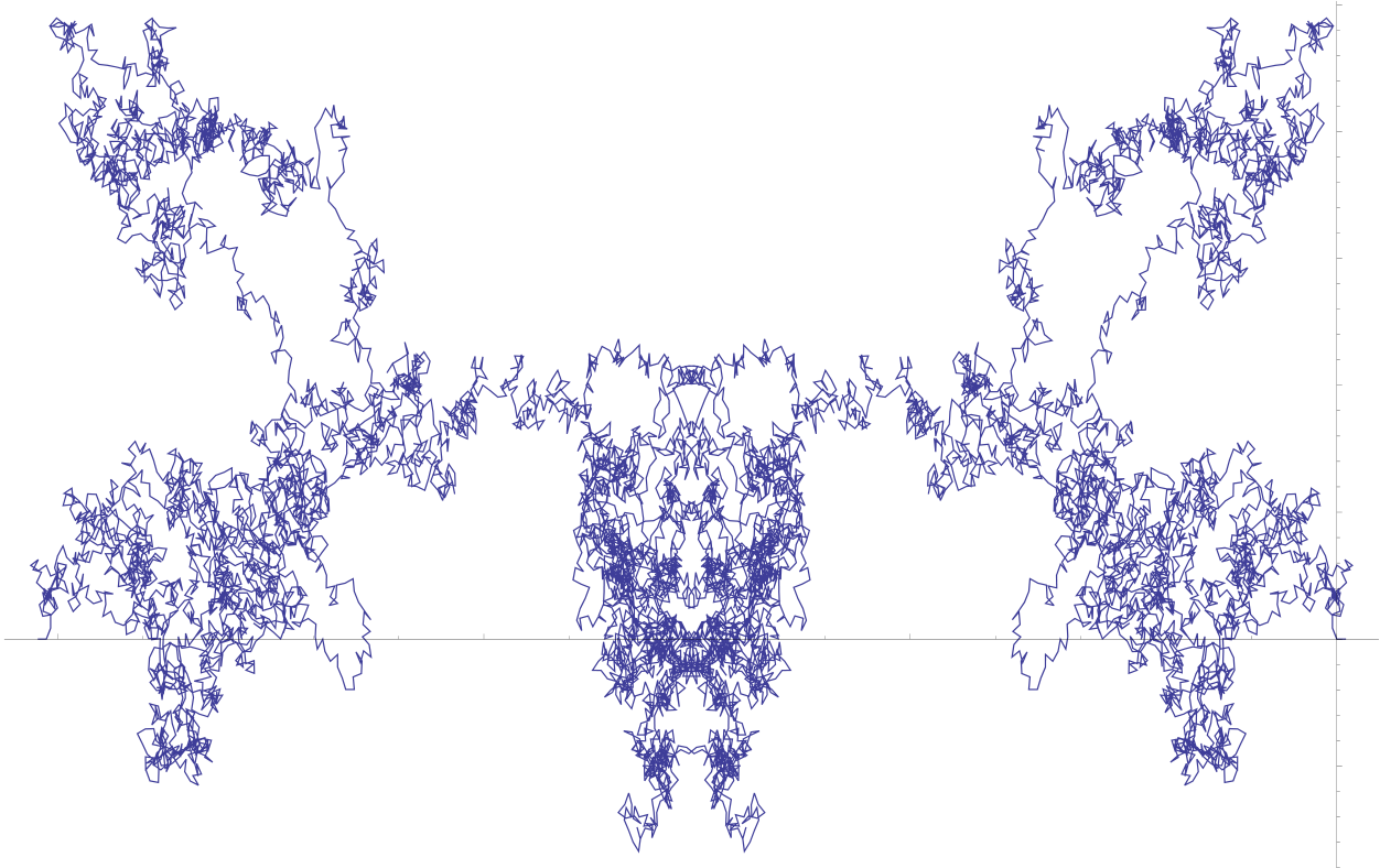
Remark 1.2. (1) Lehmer [26] and Loxton [28, 29] considered the “graphs” of various ex-ponential sums, which are the analogues of the paths t �→ Kp(t, a), but not necessarily over finite fields (see for instance the pictures in [26, p. 127] and [28, p. 154–155]). Other studies of this type are due to Dekking and Mend`es France [8] and Deshouillers [10].
In particular, in [29, p 16], Loxton mentions briefly that the paths of Kloosterman sums“seems to be absolutely chaotic”. Our result indicates one precise way in which this is true (or false).
We introduce some notation for this purpose. For each prime p, we assume given a probability space Ωp, and a family Xp = (ξp(x))x∈Fp of complex-valued random variables on p(t) for t ∈ [0, 1] by parameterizing by Ωp. We then define the associated path process KX 3
0.3
0.2
| � 0.2 | 0.2 | 0.4 | |
|---|---|---|---|
Theorem 1.1), and then we define KX p(t) for t ∈ [0, 1] as in that case, interpolating between j/(p − 1) and (j + 1)/(p − 1). We view these processes as C([0, 1])-valued random processes. We will study them in a |
|||
Remark 1.4. In Figure 1.4, we plot the function t �→ KX The complete character sums in this case are given by 10007(t, 1) for this choice of X. |
||
|---|---|---|
| Bip(a) = 1√p | x∈Fp� |
|
| distributed (on average over a). This statement was first proved by Livn´e [27]. However, his These sums were considered by Birch [3, §3], who conjectured that they are Sato-Tate- | ||
4
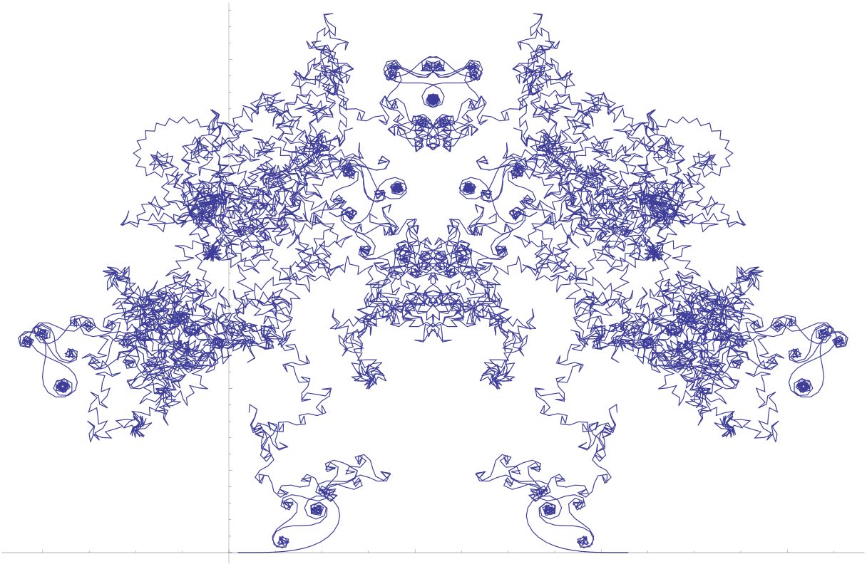
Looking at the graph for the Birch sums, one notices not only the general similarity with the graphs of Kloosterman paths (and of the random Fourier series K(t)), but also clear local differences. These are intuitively explained by the fact that the function x �→ ψp(ax + x3) is the restriction of a smooth function defined on R, and that in very short ranges (much shorter than 0 ⩽ x ⩽ pt for fixed t), the sum is well approximated by oscillatory integrals which exhibit the type of spirals and curlicues visible on the picture (see the pictures in [28]) or [10]). It would be quite interesting to find a probabilistic statement that reflects this difference between Kloosterman sums and Birch sums.
| 1⩽x⩽j� |
|
|---|
The processes (Kp(t)) on the probability spaces
p→+∞E(ϕ(Lp)) = E(ϕ(K)).
This condition is stronger than the convergence of finite-dimensional distributions. Indeed, given the convergence of finite-dimensional distributions of (Lp(t)) to those of (K(t)), one knows that convergence in law is equivalent to the weak-compactness property known as tightness (this is Prokhorov’s Theorem, see e.g. [2, Th. 7.1]).
| 1 | × | 1 | ||||
|---|---|---|---|---|---|---|
| ⩽ | ||||||
|
p − 1 | ����a ∈ F p| | max 0⩽j⩽p−1 |
√p | ���0⩽x⩽j� | ⩽ c exp(− exp(c−1A)),��� A���� |
| 5 |
| ����(α, a) ∈ F×p× F×p| | max 1⩽j⩽p−1 |
1 √p |
���1⩽x⩽j� |
|
|---|
for all A > 0. In particular, the two limits exist, and in fact they are equal.
The outline of the remainder of the paper is as follows: in Section 2, we present the proof of Theorem 1.1, and more generally of convergence of finite distributions for the situation of Theorem 1.3 (and potentially many other cases, possibly for a different random Fourier series than K(t)). In Section 3, we address the additional condition of tightness, and relate it to short exponential sums. In Section 4, we give applications, especially proving Theorem 1.6. Finally, in Section 5 we make a few remarks concerning other potential cases of convergence in law of paths of exponential sums, as well as concerning a few earlier works that have some similarity with this paper (besides those of Loxton already mentioned).
Acknowledgment. Thanks to J. Bober, L. Goldmakher, A. Granville and D. Koukoulopou-los for comments concerning their work [5]. Thanks also to J. Marklof interesting discussions 6
| Notation. For a prime p and a function ϕ : Fp −→ C, we denote by ˆϕ(h) = 1√p x∈Fp�ϕ(x)ψp(hx) |
|---|
| and the Plancherel identity | h∈Fp� | ||||
|---|---|---|---|---|---|
| x∈Fp� | ϕ1(x)ϕ2(x) = | h∈Fp� |
|
||
For any probability space (Ω, Σ,
P), we denote by P(A) the
probability of some event A, and for a
C-valued random variable X defined on Ω, we
denote by E(X) the expectation and by
V(X) = E(|X
−E(X)|2) the variance of
X, when they exist. We sometimes use different probability
spaces, but keep the same notation for all expectations and
probabilities. For σ > 0, a σ-subgaussian
(real-valued) random variable N is a random variable such
that
E(eλN) ⩽
eσ2λ2/2
confusion, if X is a random variable defined on a space Ω, we will write ∥X∥L∞(Ω) for the (essential) supremum of X.
2. Proof of convergence of finite distributions
of the random series defining K(t) converge to K(t) in law, almost surely, and in every space Lq(Ω) for 1 ⩽ q < +∞, where Ω is the probability space on which the Sato-Tate variables STh are defined. In fact, we have
(2.1) ∥Km(t)∥L∞(Ω) ≪ (log m), and
(3) The process (K(t))t∈[0,1] is almost surely continuous and almost surely nowhere differ-entiable. More precisely, it is almost surely H¨older continuous of all order α < 1/2 on [0, 1], and almost surely nowhere H¨older continuous of order 1/2.
Note that this indeed contains all statements in Theorem 1.1 (1), in particular (1.2).
| series | A(t) = | � | , | B(t) = | � |
|
||
|---|---|---|---|---|---|---|---|---|
| where | ||||||||
|
||||||||
is then given by [19, §5.5, Th. 1], and we see from [19, §7.4, Th. 3] that each of A(t) and B(t) (hence also K(t)) is α-H¨older on [0, 1] if α < 1/2. Furthermore, it follows from [19, §8.6, Th. 4] that each of A(t) and B(t) is a.s. nowhere 1/2-H¨older-continuous. |
|---|
8
Finally, from the convergence in L1(Ω) we deduce that
function of [0, t]. □
Remark 2.2. It is interesting to contrast the result with the Fourier series
Lemma 2.3. Let p ⩾ 3 be a prime and t ∈ [0, 1]. We have (2.3) √p |
|||
|---|---|---|---|
| where | αp(h; t) = 1√p | 1⩽x⩽(p−1)t� | |
| Proof. This follows from the discrete Plancherel formula, since the coefficients h �→ αp(h; t) are the discrete Fourier coefficients modulo p of the characteristic function of the interval | |||
| 1 ⩽ x ⩽ (p − 1)t. | □ | ||
From the results of Katz [21, Example 13.6], we know that for each fixed h, the Kloost-erman sums (Klp(a − h))a∈Fp are asymptotically Sato-Tate distributed. Moreover, it can be shown that they are asymptotically independent (see Lemma 2.5 below, which implies this). Since moreover αp(h; t)/√p → (e2iπht−1)/2iπh as p → +∞ (for fixed h), the expansion (2.3) is very similar to (1.1).
9
| Proposition 2.4. Let k ⩾ 1 be given, and 0 ⩽ t1 < · · · < tk ⩽ 1 be fixed. non-negative integers (n1, . . . , nk) and (m1, . . . , mk). Let | |||||
|---|---|---|---|---|---|
| Mp = | 1 | � | � | ||
| p − 1 | � | � | |||
for p ⩾ 2, where n = n1 + · · · + nk, m = m1 + · · · + mk, and the implied constant depends only on m and n. |
|||||
Since the notation may obscure the essential arithmetical point, the reader is encouraged to first read through the proof under the assumption that k = 1.
(2.4) |Kp(t, a) −˜Kp(t, a)| ⩽1√p |
|---|
for all p, a and t. We now use the formula (2.3) above, which states that
| (2.5) | ˜Kp(t, a) = 1√p | |h|<p/2� | |
|---|---|---|---|
| ���� | Kp(ti, a)niKp(ti, a) mi − | � | ˜Kp(ti, a)ni ˜Kp(ti, a) |
|
|---|---|---|---|---|
|
| ˜ | 1 | � | � | |||
|---|---|---|---|---|---|---|
| Mp = | p − 1 | � | � | |||
|
||||||
taking the ni or mi-th power. We obtain
| 1 | 1 | ||||||||
|---|---|---|---|---|---|---|---|---|---|
| p | p(m+n)/2 | p − 1 | �h1,...,hk· · ·� | nk+mk� | Klp(a − hk,l), | ||||
| where each | × | n1+m1� | Klp(a − h1,l) · · · | ||||||
hj = (hj,1, . . . , hj,nj, hj,nj+1, . . . , hj,nj+mj)
ranges over all (nj + mj)-tuples of integers hj,l in ] − p/2, p/2[ and |
|||||||||||
|---|---|---|---|---|---|---|---|---|---|---|---|
| with | 1 | �h1,...,hk· · ·� | 1⩽j⩽k� |
|
|||||||
| p = | p(m+n)/2 | ||||||||||
|
1 | � | n1+m1� | Klp(a − h1,l) · · · | nk+mk | ||||||
| p − 1 | � | � | |||||||||
where the implied constant depends only on m and n.
By (2.6), the contribution Ep of the error terms to ˜Mp is bounded by
| Xp(ti)niXp(ti) 11 mi� |
|---|
where the random variables Xp(t) are given by
| (2.8) | Xp(t) = | |h|<p/2� | αp(h; t)√p |
|
|---|---|---|---|---|
of K(t). From (2.1) and (2.2) in Proposition 2.1, we see that
|
|---|
in order to finish the proof of the proposition. |
|
|---|
|
|||||
|---|---|---|---|---|---|
|
1⩽x⩽(p−1)t� | 1 − ψp(h⌊(p − 1)t⌋) 1 − ψp(h) | |||
|
|
|---|
| − β(0; t) =⌊(p − 1)t⌋ |
|---|
12
for all t ∈ [0, 1] and p ⩾ 3. For all h such that 1 ⩽ |h| < p/2, we can then write for instance
| , | □ | ||||||
|---|---|---|---|---|---|---|---|
| − | �ψp(⌊(p − 1)t⌋h) − 1�� |
+ (ψp(h) − 1)ψp(⌊(p − 1)t⌋h) − 1 p(ψp(h) − 1) |
|||||
| and simple bounds for the three terms show that we also have | |||||||
| uniformly for all t ∈ [0, 1] and all p. Squaring and summing over h, it follows therefore that | |||||||
| E(|Xp(t) − Kp(t)|2) ≪ p−1, | |||||||
| which gives the desired bound and finishes the proof. | |||||||
S(h1, . . . , hk; p) = E�n1+m1 Zh1,l · · · � Zhk,l�+ O(p−1/2) nk+mk
where the (Zh)h∈Fp are independent random variables with Sato-Tate distributions, and the implied constant depends only on m and n.
| ( . . h p)= | 1 | � | ||
|---|---|---|---|---|
| (1 . . hk p)= | p − 1 | τ∈Fp� |
|
where
(most simply seen here because the left-hand side is unramified at 0, while the right-hand
side is ramified). Using the Goursat-Kolchin-Ribet criterion [22, §1.8], it follows that the geometric and arithmetic monodromy groups of
where A(µ), for any integer µ ⩾ 0, denotes the multiplicity of the trivial representation of
SU2 in the µ-th tensor power of its standard 2-dimensional representation, and the implied
A(µ) = E(STµ)
for any Sato-Tate distributed random-variable ST and µ ⩾ 0. Thus by reversing the com-putation, we see that
| τ∈Fp� | A(µ(τ)) = E�n1+m1 | Zh1,l · · · | nk+mk� | Zhk,l | □ | |
|---|---|---|---|---|---|---|
| where the Zh are independent and Sato-Tate distributed. | ||||||
in Theorem 1.3. We have then
Bip(a) = 1√p x∈Fp�ψp(ax + x3) |
|---|
[+τ]∗G ≃ G ⊗ L
where L is of rank 1 and τ ̸= 0. But indeed, such a sheaf L would need to be lisse on A1 (since G is). Laumon’s theory of the Fourier transform shows that G has unique slope 3/2 at
choice of non-trivial additive character modulo p, instead of ψp, and this is immediate.
3. Proof of tightness
valued processes such that Lp(0) = 0 for all p.
If there exist constants α > 0, δ > 0 and C ⩾ 0, such that for any p and any s < t in
of exponential sums:
Lemma 3.2 (Tightness and short sums). Assume that X = (ξp(x))x∈Fp is defined on Ωp, a
| |ξp(x, ω)| ⩽ 1, | |
|---|---|
�ξp(ω, h) = 1√p x∈Fp�ξp(x, ω)ψp(hx) |
|
of length (3) There exist α > 0, δ1 > 0 and δ2 > 0 such that, for any prime p, any interval I ⊂ F× p1/2−δ1⩽ |I| ⩽ p1/2+δ1, |
|---|
Remark 3.3. Note that (2) is, in practice, a special case of the main estimate of (the analogue of) Lemma 2.5 that is used to prove convergence in finite distributions. Moreover, (1) is a standard condition for the type of exponential sums we consider (typically, bounds on the Fourier transform would already follow from Weil’s theory of exponential sums in one variable).
Thus, the practical meaning of this lemma is that, once convergence of finite distributions is known “for standard reasons”, tightness becomes a consequence of the estimate (3.3). The ξp(x, ω), where the length of the sums is close to p1/2, but can be a bit smaller. latter concerns the average distribution (over ω ∈ Ωp) of short partial sums of the summands If, as one certainly expects in many cases, there exists η > 0 such that we have a uniform non-trivial individual bound
Proof of Theorem 1.3. Recall that Ωp = F×pand ξp(x, a) = ψp(ax + x3). The first condition of Lemma 3.2 is then clear. The second condition holds by (the analogue for the Birch sums of) Lemma 2.5. For (3), the point is that individual bounds for sums over intervals of polynomials of rather short length are known, from methods such as Weyl differencing, so we can use the argument indicated in the previous remark.
Precisely, by Weyl’s method, one gets
| p | 1/4 | |||
|---|---|---|---|---|
| � | ψp( +) ≪ ||�|I|+ | |I|3 | ||
for 1 ⩽ |I| < p and for any ε > 0, where the implied constant depends only on ε (see, e.g., [18, Lemma 20.3]). In particular, if we assume that p5/12⩽ |I| ⩽ p7/12 16 |
||||
and selecting α large enough, we obtain the desired estimate (3.3). p − 1 ���� 1√p�ψp(ax + x3)
|
□ |
| Proof of Theorem 1.5. As before, it only remains to prove (3.3) for the process (Kp(t)) (here the summands ψp(α(ax + ¯x)) are parameterized by x ∈ F×the fourth moment (just as Kloosterman did for the full interval to get the first non-trivial p). We take α = 4 and compute | |
| 1 |
|
� 1 x1 | −1 x3 | |||||||||||||
|---|---|---|---|---|---|---|---|---|---|---|---|---|---|---|---|---|
| (p − 1)2 |
|
�α | −1 x4 | |||||||||||||
| 1 | � | ψp(αa(x1 + x2 − x3 − x4)). | ||||||||||||||
| × | � | |||||||||||||||
| 1 | x1+x2=x3+x4� � | 1 | � | ψ | 1 |
|
1 | 1 |
|
|||||
|---|---|---|---|---|---|---|---|---|---|---|---|---|---|---|
| p(p − 1) | p − 1 | α∈F×� | p | �x1 | −x3 | −x4 | �� | |||||||
| and then to | 1 |
|
||||||||||||
| (p − 1)2 | ||||||||||||||
|
||||||||||||||
| 1 | 1 | � |
|
= | 1 | ψ | 1 | + 1 | 1 | 1 | |||||||
|---|---|---|---|---|---|---|---|---|---|---|---|---|---|---|---|---|---|
| p − 1 |
|
� |
|
p(p − 1) | x1+x2=x3+x4� � | p | �x1 | x2 | −x3 | −x4 |
|
||||||
| + O(|I|4p−3). | |||||||||||||||||
| Since the number of points of summation is about |I|3(because I is an interval), thisleads to a bound p−1/2when |I| is itself p1/2. The difficulty is therefore that we must get some cancellation in the exponential sum over the xi’s to avoid the extra average over additive | |||||||||||||||||
| h̸=−1� | e(ht) − 1 2iπh |
|
|
||||||||
|---|---|---|---|---|---|---|---|---|---|---|---|
| 1 | 1 | � |
|
1 |
|
||||||
| p − 1 |
|
� | p(p − 1) | x−1 1+x−1� �2=x−1 3+x−1 | |||||||
| + O(|I|4p−3), | |||||||||||
| and a result of Bourgain and Garaev [6, Th. 1] shows that the number of points of summation is ≪ |I|8/3+εfor any ε > 0, provided |I| ⩽ p3/4, which is enough to verify the hypothesis of Lemma 3.2. | |||||||||||
be the discontinuous analogue of Lp(t). We first reduce the problem to proving a moment |
|---|
| (3.4) |
|
|---|---|
for any α > 0 and all primes p, which is fine as soon as α > 2. |
|
the analogue of the random variables in (2.8) for intervals 0 ⩽ j ⩽ pt instead of 1 ⩽ j ⩽(p − 1)t. For s ⩽ t in [0, 1], we will also denote by I the interval ps ⩽ x ⩽ pt, of length |I| ≍ |t − s|p (recall that |s − t| ⩾ 1/p now). |
|---|
This indeed follows from the assumption (3.2) of Lemma 3.2, by the same method used in the proof of convergence of finite distributions.
Next, we claim that there exists C ⩾ 0 such that, for all s, t in [0, 1] and all p, we have
| (3.7) | |||||||
|---|---|---|---|---|---|---|---|
| (in particular, the sequence (Xp(t))t∈[0,1] is itself tight by Kolmogorov’s criterion). Indeed, we can use the fact that | |||||||
| Xp(t) − Xp(s) = | |h|<p/2� | ||||||
| is σp-subgaussian, where | |||||||
p |
|h|<p/2� | |α′p(h; t) − α′p(h; s)|2 = 1 | ps⩽x⩽pt� |
|
|||
| for all s and t such that |t − s| ⩾ p−1/(2(1+η)), where the implied constant depends only on ε. For suitable η > 0 and ε > 0, this gives | |
|---|---|
| (3.8) | |
|˜Lp(t, ω) −˜Lp(s, ω)| ⩽|I|√p ≪ p1/2|t − s| ≪ p−δ1 |
|
(3.10) E(|˜Lp(t) −˜Lp(s)|α) ≪ p−1/2−δ2≪ |t − s|(1/2+δ2)/(1/2+δ1)⩽ |t − s|1+δ′′for some δ′′> 0, since we assumed that δ2 > δ1.
combination of the three bounds, and we have a suitable inequality for each range. The We can now combine (3.8), (3.9) and (3.10). All ranges of |t − s| are covered by the


