

Eigenvalues & Diagonalization
In this lab, we're going to learn how to use MATLAB to compute the eigenvalues, eigenvectors, and determinants of matrices. Then we'll use these new mathematical tools to revisit old problems from a new perspective.
Determinants
As you should be aware by now, there is a nice formula for calculating the determinant of a 2×2 matrix. Even the 3×3 case is not too hard. But as the size of a matrix increases, the determinant calculation gets much more complicated. This is where MATLAB comes in.
ans =
76
Use MATLAB to compute the determinants of the matrices A+B, A-B, AB, A-1, and BT. (Recall that in MATLAB, BT is written as B'.)
Which of the above matrices are not invertible? Explain your reasoning.
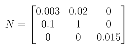
Use det() to calculate the determinant of N100. Based on this information, do you think that N100 is invertible?
Eigenvalues and Eigenvectors
>> b = eig(B)
b =
Thus we see that the eigenvalues are 1, 8, 3, and 2; there are four eigenvalues because our matrix is 4×4. (As an aside, note that we can quickly compute the determinant of B with this information: it's just the product of the eigenvalues.)
If we want to compute the eigenvalues and corresponding eigenvectors all in one step, we can simply use the following command:
0 0.6931 0.9428 0.3630
0 0 0 0.1089
0 0 0 2
The matrix P here has the eigenvectors of B as its columns, and the diagonal matrix D has the corresponding eigenvectors along the diagonal. This means, for instance, that the second column of P is an eigenvector for the eigenvalue 8, which is the second entry along the diagonal of D.
If we've done everything correctly, we should get 0, since x is supposed satisfy the equation Bx = 8x.
Now let's explore one of the interesting properties of these eigenvalue and eigenvector matrices.
Determine whether V is invertible by looking at the eigenvalues. Explain your reasoning.
Use MATLAB to evaluate P-1VP. What do you notice?
Diagonalization
Not every matrix is diagonalizable. In order to diagonalize an n×n matrix, we need to find n eigenvectors of that matrix that form a basis of Rn. These n linearly independent eigenvectors form the columns of P, and then the entries of D are the matching eigenvalues. If we can't find a basis consisting only of eigenvectors, then the matrix isn't diagonalizable.
Theorem: If an n×n matrix has n distinct eigenvalues, then the matrix is diagonalizable.
Use MATLAB to find an invertible matrix P and a diagonal matrix D such that PDP-1 = F.
Use MATLAB to compare F10 and PD10P-1.
Electoral Trends Revisited
In California, when you register to vote, you declare a party affiliation. Suppose we have just four political parties: Democrats, Republicans, Independents, and Libertarians. Party registration data is public, so we can track what fraction of the voters in each party switch to a different party from one election to the next. Let's say we look up Democratic Party registration data and discover the following: 81% of Democrats remain Democrats, 9% become Republicans, 6% re-register as Independents, and 4% become Libertarians. We can do the same kind of calculation for the other three parties and then organize our data into a table:
| Democrats | Republicans | Independents | Libertarians | |
|---|---|---|---|---|
| Democrats | 0.81 | 0.08 | 0.16 | 0.10 |
| Republicans | 0.09 | 0.84 | 0.05 | 0.08 |
| Independents | 0.06 | 0.04 | 0.74 | 0.04 |
| Libertarians | 0.04 | 0.04 | 0.05 | 0.78 |
In this table, we've put our results in the columns, so the numbers reflect the proportion of voters in that column's political party who switch to the party listed to the left. For example, the entry in the "Republicans" row and the "Independents" column tells us that 5% of Independents become Republicans each electoral cycle. We're going to assume that these numbers do not change from one election to the next—not a very realistic assumption, but good enough for our simple model.
>> P = [0.8100 0.0800 0.1600 0.1000;
0.0900 0.8400 0.0500 0.0800;
For this exercise, we'll need to introduce the concept of limits. Many of you will have already seen limits in pre-calculus or calculus classes. A rough intuitive definition of limit is this: a limit is a number that a function "approaches" when the numbers you plug in to that function get close to a certain value. So if we say, "The limit of the function f(x) when x approaches 2 is 5," that means we can make f(x) as close as we like to the value 5 by choosing values for x that are closer and closer to 2.
You can also speak of limits of sequences of numbers: if we have a sequence {an}, to say that the limit of this sequence is L is to say that however close you ask me to get to L, I can find a term in the sequence so that all the subsequent terms are that close to L. Formally, the criterion is that for every positive number ε (no matter how small), there is an index N such that for each term xn after xN, the difference between L and xn is less than ε.
Using MATLAB, multiply L by Q and Q-1 (on the appropriate sides) to compute P∞, the limit as n tends to infinity of Pn. Store the answer in a variable called Pinf.
Now use MATLAB to compute P∞x0. How does your answer compare to the results you saw in the second part of the exercise from last lab?
PageRank Revisited
Now we've recast the phenomenon behind PageRank as one involving eigenvalues, eigenvectors, and iteration of the matrix L (i.e., raising L to large powers). Specifically, if we take n to be large enough, then Lnr0 will approach the solution we're looking for.
0,0,0,0,0,0,0,1;
0,1/2,0,0,0,0,1,0;
0,0,0,1,0,0,0,0;]
Let e0 = (1, 1, 1, 1, 1, 1, 1, 1)T, and define en+1 = Len (which is the same as saying en = Lne0). Use MATLAB to compute e10. How large must n be so that each entry of en changes by less than 1% when we increase n by 1? [Don't try to get an exact value, just try to get a value for n that's big enough.]
Conclusion
We've now learned how to use MATLAB to compute determinants, eigenvalues, and eigenvectors, and we've used these tools to diagonalize matrices. We've also studied how these things can be applied to study fairly complex models using iteration.


