

The load must equal the true stress times the actual area
This module outlines the basic mechanics of elastic response — a physical phenomenon that materials often (but do not always) exhibit. An elastic material is one that deforms immediately upon loading, maintains a constant deformation as long as the load is held constant, and returns immediately to its original undeformed shape when the load is removed. This module will also introduce two essential concepts in Mechanics of Materials: stress and strain.
Tensile strength and tensile stress
1
magnitude of its cross-sectional area. This notion is reasonable when one considers the strength to arise from the number of chemical bonds connecting one cross section with the one adjacent to it as depicted in Fig. 2, where each bond is visualized as a spring with a certain stiffness and strength. Obviously, the number of such bonds will increase proportionally with the section’s area1. The axial strength of a piece of blackboard chalk will therefore increase as the square of its diameter. In contrast, increasing the length of the chalk will not make it stronger (in fact it will likely become weaker, since the longer specimen will be statistically more likely to contain a strength-reducing flaw.)
the “proportionate” strength of the famous arachnid mentioned weekly in the SpiderMan comic strip is mostly just this same size effect. There’s nothing magical about the muscular strength of insects, but the ratio of L2to L3works in their favor when strength per body weight is reckoned. This cautions us that simple scaling of a previously proven design is not a safe design procedure. A jumbo jet is not just a small plane scaled up; if this were done the load-bearing components would be too small in cross-sectional area to support the much greater loads they would be called upon to resist.
| (1) |
|---|
NS =�7.86 cm3 · 6.023 × 1023 atoms 55.85 mol g �2 = 1.9 × 10¹⁵ atoms cm2
NS ≈ 1015 atom cm2 is true for many materials.
called Pascals, or Pa) in the SI system and lb/in2(or psi) in units still used commonly in the United States.
Example 1
A0 =Pf
σfAll we need do is look up the value of σf for the material, and substitute it along with the value of 10,000 lb for Pf, and the problem is solved.
1
We probably wouldn’t order rod of exactly 0.38 in, as that would be an oddball size and thus too d =� 4A π=�πσf 4Pf = π × 600 × 106(N/m2) × 1.449 × 10−4 4 × 10000(lb) � lb/in2 N/m2� = 0.38 in
2
The tensile stress, the force per unit area acting on a plane transverse to the applied load, is a fundamental measure of the internal forces within the material. Much of Mechanics of Materials is concerned with elaborating this concept to include higher orders of dimensionality, working out methods of determining the stress for various geometries and loading conditions, and predicting what the material’s response to the stress will be.
Example 2
W(y) = γV = γAy
4
The length of rod that is just on the verge of breaking under its own weight can now be found by letting y = L (the highest stress occurs at the top), setting σ(L) = σf, and solving for L:
σf = γL ⇒ L =σf
γ
It is important to distinguish stiffness, which is a measure of the load needed to induce a given deformation in the material, from the strength, which usually refers to the material’s resistance to failure by fracture or excessive deformation. The stiffness is usually measured by applying relatively small loads, well short of fracture, and measuring the resulting deformation. Since the deformations in most materials are very small for these loading conditions, the experimental problem is largely one of measuring small changes in length accurately.
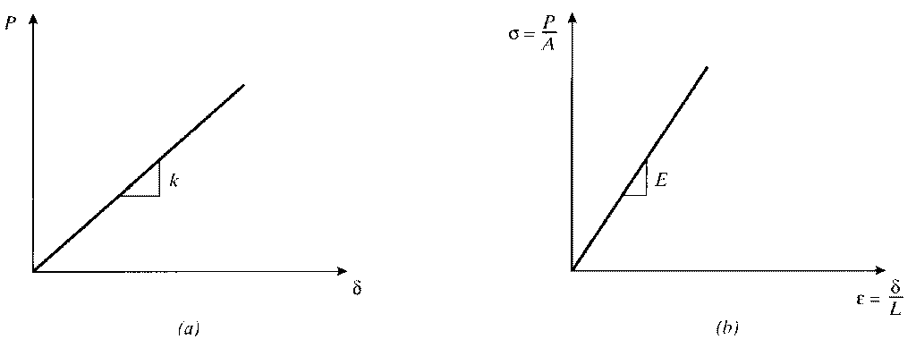
Hooke3made a number of such measurements on long wires under various loads, and observed that to a good approximation the load P and its resulting deformation δ were related linearly as long as the loads were sufficiently small. This relation, generally known as Hooke’s Law, can be written algebraically as
3Robert Hooke (1635–1703) was a contemporary and rival of Isaac Newton. Hooke was a great pioneer in mechanics, but competing with Newton isn’t easy.
5
| P | (5) | |
|---|---|---|
| A0 |
The constant of proportionality E, called Young’s modulus5or the modulus of elasticity, is one of the most important mechanical descriptors of a material. It has the same units as stress, Pa or psi. As shown in Fig. 6, Hooke’s law can refer to either of Eqns. 3 or 6.
|
(8) |
|---|
Note that the stress σ = P/A developed in a tensile specimen subjected to a fixed load is independent of the material properties, while the deflection depends on the material property E. Hence the stress σ in a tensile specimen at a given load is the same whether it’s made of steel or polyethylene, but the strain ϵ would be different: the polyethylene will exhibit much larger strain and deformation, since its modulus is two orders of magnitude less than steel’s.
In Example 1, we found that a steel rod 0.38′′in diameter would safely bear a load of 10,000 lb. Now let’s assume we have been given a second design goal, namely that the geometry requires that we use a rod 15 ft in length but that the loaded end cannot be allowed to deflect downward more than 0.3′′when the load is applied. Replacing A in Eqn. 8 by πd2/4 and solving for d, the diameter for a given δ is
d = 2�πδE
PL
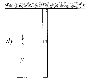
Figure 7: Deformation of a column under its own weight.
can also be written
7
However, this analysis assumes Hooke’s law holds over the entire range of stresses from zero to fracture. This is not true for many materials, including carbon steel, and later modules will address materials response at high stresses.
A material that obeys Hooke’s Law (Eqn. 6) is called Hookean. Such a material is elastic according to the description of elasticity given in the introduction (immediate response, full recovery), and it is also linear in its relation between stress and strain (or equivalently, force and deformation). Therefore a Hookean material is linear elastic, and materials engineers use these descriptors interchangeably. It is important to keep in mind that not all elastic materials are linear (rubber is elastic but nonlinear), and not all linear materials are elastic (viscoelastic materials can be linear in the mathematical sense, but do not respond immediately and are thus not elastic).
2. Two rods, one of nylon and one of steel, are rigidly connected as shown. Determine the stresses and axial deformations when an axial load of F = 1 kN is applied.
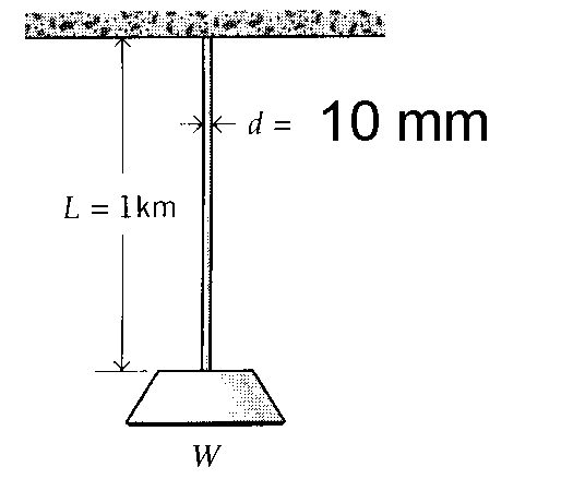
3. A steel cable 10 mm in diameter and 1 km long bears a load in addition to its own weight of W = 150 N. Find the total elongation of the cable.
Prob. 2
8. A tapered column of modulus E and mass density ρ varies linearly from a radius of r1 to r2 in a length L, and is hanging from its broad end. Find the total deformation due to the weight of the bar.
9. A rod of circular cross section hangs under the influence of its own weight, and also has an axial load P suspended from its free end. Determine the shape of the bar, i.e. the function r(y) such that the axial stress is constant along the bar’s length.
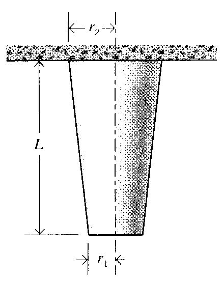
Prob. 8
10
ATOMISTIC BASIS OF ELASTICITY
For most materials, the amount of stretching experienced by a tensile specimen under a small fixed load is controlled in a relatively simple way by the tightness of the chemical bonds at the atomic level, and this makes it possible to relate stiffness to the chemical architecture of the material. This is in contrast to more complicated mechanical properties such as fracture, which are controlled by a diverse combination of microscopic as well as molecular aspects of the material’s internal structure and surface. Further, the stiffness of some materials — notably rubber — arises not from bond stiffness but from disordering or entropic factors. Some principal aspects of these atomistic views of elastic response are outlined in the sections to follow.
Energetic effects
3. Covalent materials, such as diamond and polyethylene, in which atomic orbitals overlap to form a region of increased electronic charge to which both nuclei are attracted. This bond is directional, with each of the nuclear partners in the bond feeling an attraction to the negative region between them but not to any of the other atoms nearby.
In the case of ionic bonding, Coulomb’s law of electrostatic attraction can be used to develop simple but effective relations for the bond stiffness. For ions of equal charge e the attractive force fattr can be written:
| Uattr = | � | (2) | |
|---|---|---|---|
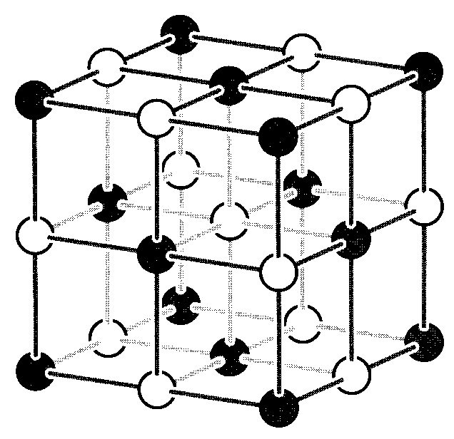
Figure 1: The interpenetrating cubic NaCl lattice.
2
where A = 1.747558 · · · is the result of the previous series, called the Madelung constant1. Note that it is not sufficient to consider only nearest-neighbor attractions in computing the bonding energy; in fact the second term in the series is larger in magnitude than the first. The specific value for the Madelung constant is determined by the crystal structure, being 1.763 for CsCl and 1.638 for cubic ZnS.
Figure 2: The bond energy function.
As shown in Fig. 2, the total binding energy of one ion due to the presence of all others is then the sum of the attractive and repulsive components:
| (5) |
|---|
Example 1
When the separation between two adjacent ions is increased by an amount δ, the strain is ϵ = δ/r0. The differential strain corresponding to a differential displacement is then
dϵ =dr
r0
| d | �ACe2 |
|
|||
|---|---|---|---|---|---|
| dr |
E = (n − 1)ACe2
r4 0the resulting value of n is too low. A better but slightly more complicated approach is to use hydrostatic
2See the Module on Crystallographic Notation for a review of this nomenclature.
The stiffnesses of metallic and covalent systems will be calculated differently than the method used above for ionic crystals, but the concept of electrostatic attraction applies to these non-ionic systems as well. As a result, bond energy functions of a qualitatively similar nature result from all these materials. In general, the “tightness” of the bond, and hence the elastic modulus E, is related to the curvature of the bond energy function. Steeper bond functions will also be deeper as a rule, so that within similar classes of materials the modulus tends to correlate with the energy needed to rupture the bonds, for instance by melting. Materials such as tungsten that fill many bonding and few antibonding orbitals have very deep bonding functions3, with correspondingly high stiffnesses and melting temperatures, as illustrated in Fig. 4. This correlation is obvious in Table 1, which lists the values of modulus for a number of metals, along with the values of melting temperature Tm and melting energy ∆H.
Table 1: Modulus and bond strengths for transition metals.
addition of heat, the system oscillates between the positions labeled A′and B′with an average separation distance r′0. Since the curve is anharmonic, the average separation distance is now greater than before, so the material has expanded or stretched. To a reasonable approximation,
the relative thermal expansion ∆L/L is often related linearly to the temperature rise ∆T, and
| ∆L | (7) | |
|---|---|---|
| L |
Figure 5: Anharmonicity of the bond energy function.
Example 2
If the bar were free to expand, it would increase in length by an amount given by Eqn. 7. Clearly,
the rigid supports have to push on the bar – i.e. put in into compression – to suppress this expansion.
σ = −αLE∆T
The minus sign in this result reminds us that a negative (compressive) stress is induced by a positive temperature change (temperature rises.)
σ = −αLE∆T
Here the temperature change ∆T is negative if the glass is going from hot to cold, so the stress is positive (tensile). If the glass is not to fracture by thermal shock, this stress must be less than the ultimate tensile strength σf; hence the maximum allowable temperature difference is
The internal energy as given by the function U(r) is sufficient to determine the atomic positions in many engineering materials; the material “wants” to minimize its internal energy, and it does this by optimizing the balance of attractive and repulsive electrostatic bonding forces.
7
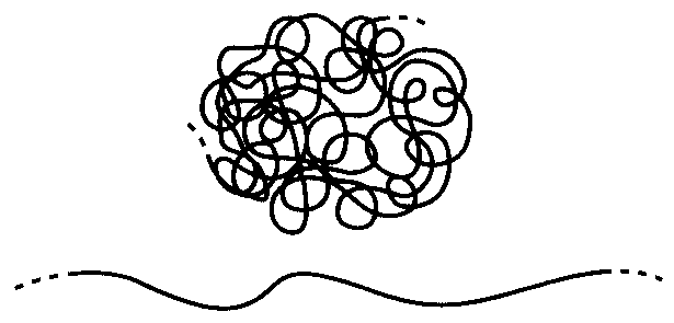
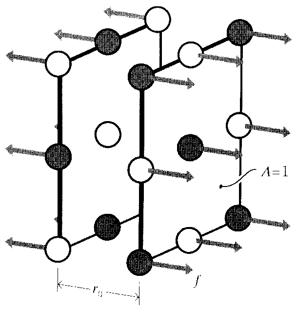
Figure 8: Conformational change in polymers.
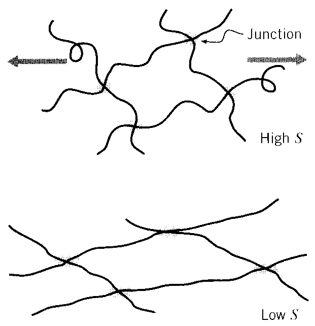
When we stretch a rubber band, the molecules in its interior become extended because they are crosslinked by chemical or physical junctions as shown in Fig. 9. Without these links, the molecules could simply slide past one another with little or no uncoiling. “Silly Putty ” is an example of uncrosslinked polymer, and its lack of junction connections cause it to be a viscous fluid rather than a useful elastomer that can bear sustained loads without continuing flow. The crosslinks provide a means by which one molecule can pull on another, and thus establish load transfer within the materials. They also have the effect of limiting how far the rubber can be stretched before breaking, since the extent of the entropic uncoiling is limited by how far the material can extend before pulling up tight against the network of junction points. We will see below that the stiffness of a rubber can be controlled directly by adjusting the crosslink density, and this is an example of process-structure-property control in materials.
9
the wheel so that a heat lamp shines on the bands to the right or left of the hub. As the bands warm up, they contract. This pulls the rim closer to the hub, causing the wheel to become unbalanced. It will then rotate under gravity, causing the warmed bands to move out from under the heat lamp and be replaced other bands. The process continues, and the wheel rotates in a direction opposite to what would be expected were the spokes to expand rather than contract on heating.
When pressure-volume changes are not significant, the competition between internal energy and entropy can be expressed by the Helmholtz free energy A = U − TS, where T is the temperature and S is the entropy. The system will move toward configurations of lowest free energy, which it can do either by reducing its internal energy or by increasing its entropy. Note that the influence of the entropic term increases explicitly with increasing temperature. With certain thermodynamic limitations in mind (see Prob. 5), the mechanical work dW = F dL done by a force F acting through a differential displacement dL will produce an increase in free energy given by
F dL = dW = dU − T dS (8)
| F =dW dL= | �∂U | �T,V | − T | �∂S | (9) |
|---|
We begin by writing an expression for the conformation, or shape, of the segment of polymer molecule between junction points as a statistical probability distribution. Here the length of the segment is the important molecular parameter, not the length of the entire molecule. In the simple form of this theory, which turns out to work quite well, each covalently bonded segment is idealized as a freely-jointed sequence of n rigid links each having length a.

well known to seasoned test-takers. The most probable end-to-end distance is seen to be zero,�
the bond length a; specifically it turns out that β = 3/2n/a. This is the “bell-shaped curve”which is expected because the chain will end up a given distance to the left (or up, or back) of the origin exactly as often as it ends up the same distance to the right.
11
shown (see Prob. 8) that the distance r2 0is related to the number of bonds n in the segment and
the bond length a by r2 0= na2. Making these substitutions and simplifying, we have
are related to corresponding changes in thermodynamic entropy by the “Boltzman relation” as
∆S = k ln Ω2
This is the entropy change for one segment. If there are N chain segments per unit volume, the
total entropy change per unit volume ∆SV is just N times this quantity:
2 � λ2 x+ λ2 y+ λ2 z− 3� (12)
The quantity ∆WV is therefore the strain energy per unit volume contained in an ideal rubber
force microscopy (AFM). At low to moderate extensions, most polymer chains behave as ideal, entropic,
random coils; i.e. molecular rubber bands. This is shown in Fig. 12, which displays AFM data (re-
local environmental effects (e.g. electrostatic interactions, solvent quality, etc.). In addition, force spec-
troscopy can be used to measure noncovalent, physisorption forces of single polymer chains on surfaces
lets us compute the transverse contractions λy and λz which accompany the stretch λx. An
12
Setting this to zero gives
λxλyλz = 1 (13)
| F =dW dL= d(V ∆WV ) L0 dλ | = A0 | NkT | λ2 |
|
|---|---|---|---|---|
| 2 |
Clearly, the parameter NkT is related to the stiffness of the rubber, as it gives the stress σ needed to induce a given extension λ. It can be shown (see Prob. 10) that the initial modulus— the slope of the stress-strain curve at the origin — is controlled by the temperature and the crosslink density according to E = 3NkT.
Crosslinking in rubber is usually done in the “vulcanizing” process invented by Charles Goodyear in 1839. In this process sulfur abstracts reactive hydrogens adjacent to the double
The Young’s modulus of a rubber is measured at E = 3.5 MPa for a temperature of T = 300◦K. The molar crosslink density is then
| N = |
|
|---|
A person with more entrepreneurial zeal than caution wishes to start a bungee-jumping company, and naturally wants to know how far the bungee cord will stretch; the clients sometimes complain if the cord fails to stop them before they reach the asphalt. It’s probably easiest to obtain a first estimate from an energy point of view: say the unstretched length of the cord is L0, and that this is also the distance the jumper free-falls before the cord begins to stretch. Just as the cord begins to stretch, the the jumper has lost an amount of potential energy wL0, where w is the jumper’s weight. The jumper’s velocity at this time could then be calculated from (mv2)/2 = wL0 if desired, where m = w/g is the jumper’s mass and g is the acceleration of gravity. When the jumper’s velocity has been brought to zero by the cord (assuming the cord doesn’t break first, and the ground doesn’t intervene), this energy will now reside as entropic strain energy within the cord. Using Eqn. 12, we can equate the initial and final energies to obtain
| A0E= 1 | �λ2+ 2 λ− 3 |
|---|
Taking a typical design case for illustration, say the desired extension ratio is taken at λ = 3 for a rubber cord of initial modulus E = 100 psi; this stops the jumper safely above the pavement and is verified
14
Note that the stress-strain response for rubber elasticity is nonlinear, and that the stiffness as given by the stress needed to produce a given deformation is predicted to increase with increasing temperature. This is in accord with the concept of more vigorous wriggling with a statistical bias toward the more disordered state. The rubber elasticity equation works well at lower extensions, but tends to deviate from experimental values at high extensions where the segment configurations become nongaussian.
Deviations from Eqn. 14 can also occur due to crystallization at high elongations. (Rubbers are normally noncrystalline, and in fact polymers such as polyethylene that crystallize readily are not elastomeric due to the rigidity imparted by the crystallites.) However, the decreased entropy that accompanies stretching in rubber increases the crystalline melting temperature according to the well-known thermodynamic relation
2. Using Eqn. 6 to write the parameter B in terms of the equilibrium interionic distance r0, show that the binding energy of an ionic crystal, per bond pair, can be written as
15
| K = − | dp (dV )/V |
|---|
(a) Use the relation dU = pdV for the energy associated with pressure acting through a small volume change to show
| K | = | � | d2U | �V =V0 | = | 9c2N2r2 · d dr | � 1 r2 | dU | |
|---|---|---|---|---|---|---|---|---|---|
| V0 | dV2 | dr |
(c) Carry out the indicated differentiation of the expression for binding energy to obtain the expression
ACe2
4. Complete the spreadsheet below, filling in the values for repulsion exponent n and lattice
| type | r0 (pm) | A | n | U(kJ/mol) | ||
|---|---|---|---|---|---|---|
| LiF | 201.4 | 6.710e+01 | 1.750 |
|
||
| NaCl | 282.0 | 2.400e+01 | 1.750 |
|
||
| KBr | 329.8 | 1.480e+01 | 1.750 |
6. Show that the temperature dependence of the force needed to hold a tensile specimen at fixed length as the temperature is changed (neglecting thermal expansion effects) is related to the dependence of the entropy on extension as
| �∂F | �L | = − | �∂S |
|
|---|
17
9. Evalute the temperature rise in a rubber specimen of ρ = 1100 kg/m3, c = 2 kJ/kg·K, NkT = 500 kPa, subjected to an axial extension λ = 4.
| σx = NkT | � | λx − | 1 | |
|---|---|---|---|---|
| λ3xλ2y |
and based on the deformed dimensions
| tan φ′= |
|---|
15. Before stretching, the molecular segments in a rubber sheet are assumed to be distributed uniformly over all directions, so the the fraction of segments f(φ) oriented in a particular range of angles dφ is
f(φ) =dA A= 2πr2 sin φ dφ
Using the result of the previous problem, plot the orientation function f as a function of
the extension ratio λ.
Introduction
This module introduces basic concepts of stiffness and strength underlying the mechanics of fiber-reinforced advanced composite materials. This aspect of composite materials technology is sometimes terms “micromechanics,” because it deals with the relations between macroscopic engineering properties and the microscopic distribution of the material’s constituents, namely the volume fraction of fiber. This module will deal primarily with unidirectionally-reinforced continuous-fiber composites, and with properties measured along and transverse to the fiber direction.
1F.P. Gerstle, “Composites,” Encyclopedia of Polymer Science and Engineering, Wiley, New York, 1991. Here E is Young’s modulus, σb is breaking stress, ϵb is breaking strain, and ρ is density.
1
Of course, these materials are not generally usable as fibers alone, and typically they are impregnated by a matrix material that acts to transfer loads to the fibers, and also to pro-tect the fibers from abrasion and environmental attack. The matrix dilutes the properties to some degree, but even so very high specific (weight-adjusted) properties are available from these materials. Metal and glass are available as matrix materials, but these are currently very ex-pensive and largely restricted to R&D laboratories. Polymers are much more commonly used, with unsaturated styrene-hardened polyesters having the majority of low-to-medium perfor-mance applications and epoxy or more sophisticated thermosets having the higher end of the market. Thermoplastic matrix composites are increasingly attractive materials, with processing difficulties being perhaps their principal limitation.
Stiffness
Figure 2: Loading parallel to the fibers.
Consider a typical region of material of unit dimensions, containing a volume fraction Vf of fibers all oriented in a single direction. The matrix volume fraction is then Vm = 1 − Vf. This region can be idealized as shown in Fig. 2 by gathering all the fibers together, leaving the matrix to occupy the remaining volume — this is sometimes called the “slab model.” If a stress σ1 is applied along the fiber direction, the fiber and matrix phases act in parallel to support the load. In these parallel connections the strains in each phase must be the same, so the strain ϵ1 in the fiber direction can be written as:
|
|
(1) |
|---|
Figure 4 shows the functional form of the parallel (Eqn. 1) and series (Eqn. 2) predictions for the fiber- and transverse-direction moduli.
The prediction of transverse modulus given by the series slab model (Eqn. 2) is considered unreliable, in spite of its occasional agreement with experiment. Among other deficiencies the
In more complicated composites, for instance those with fibers in more than one direction or those having particulate or other nonfibrous reinforcements, Eqn. 1 provides an upper bound to the composite modulus, while Eqn. 2 is a lower bound (see Fig. 4). Most practical cases will be somewhere between these two values, and the search for reasonable models for these intermediate cases has occupied considerable attention in the composites research community. Perhaps the most popular model is an empirical one known as the Halpin-Tsai equation2, which can be written in the form:
|
(3) |
|---|
The stress σ∗is the stress in the matrix, which is given by ϵfbEm. This relation is linear in Vf, rising from σ∗to the fiber breaking strength σfb = Efϵfb. However, this relation is not realistic at low fiber concentration, since the breaking strain of the matrix ϵmb is usually substantially greater than ϵfb. If the matrix had no fibers in it, it would fail at a stress σmb = Emϵmb. If the fibers were considered to carry no load at all, having broken at ϵ = ϵfb and leaving the matrix
2c.f. J.C.. Halpin and J.L. Kardos, Polymer Engineering and Science, Vol. 16, May 1976, pp. 344–352.
σb = (1 − Vf)σmb
Since the breaking strength actually observed in the composite is the greater of these two expressions, there will be a range of fiber fraction in which the composite is weakened by the addition of fibers. These relations are depicted in Fig. 6.References
1. Ashton, J.E., J.C. Halpin and P.H. Petit, Primer on Composite Materials: Analysis,Technomic Press, Westport, CT, 1969.
6. Roylance, D., Mechanics of Materials, Wiley & Sons, New York, 1996.
5
Figure 6: Strength of unidirectional composite in fiber direction.
Problems
4. What is the maximum fiber volume fraction Vf that could be obtained in a unidirectionally reinforced with optimal fiber packing?
5. Using the slab model and assuming uniform strain in the matrix, show the transverse
or in terms of compliances
C2 = CfVf + CmVm
Introduction
Stress-strain curves are an extremely important graphical measure of a material’s mechanical properties, and all students of Mechanics of Materials will encounter them often. However, they are not without some subtlety, especially in the case of ductile materials that can undergo sub-stantial geometrical change during testing. This module will provide an introductory discussion of several points needed to interpret these curves, and in doing so will also provide a preliminary overview of several aspects of a material’s mechanical properties. However, this module will not attempt to survey the broad range of stress-strain curves exhibited by modern engineering materials (the atlas by Boyer cited in the References section can be consulted for this). Several of the topics mentioned here — especially yield and fracture — will appear with more detail in later modules.
A0 |
|
(1) |
|---|
1Stress-strain testing, as well as almost all experimental procedures in mechanics of materials, is detailed by standards-setting organizations, notably the American Society for Testing and Materials (ASTM). Tensile testing of metals is prescribed by ASTM Test E8, plastics by ASTM D638, and composite materials by ASTM D3039.
1
In the early (low strain) portion of the curve, many materials obey Hooke’s law to a reason-able approximation, so that stress is proportional to strain with the constant of proportionality being the modulus of elasticity or Young’s modulus, denoted E:
σe = Eϵe (2)
when the load is removed, so the proportional limit is often the same as or at least close to the materials’s elastic limit. Elasticity is the property of complete and immediate recovery from an imposed displacement on release of the load, and the elastic limit is the value of stress at which the material experiences a permanent residual strain that is not lost on unloading. The residual strain induced by a given stress can be determined by drawing an unloading line from the highest point reached on the se - ee curve at that stress back to the strain axis, drawn with a slope equal to that of the initial elastic loading line. This is done because the material unloads elastically, there being no force driving the molecular structure back to its original position.
A closely related term is the yield stress, denoted σY in these modules; this is the stress needed to induce plastic deformation in the specimen. Since it is often difficult to pinpoint the exact stress at which plastic deformation begins, the yield stress is often taken to be the stress needed to induce a specified amount of permanent strain, typically 0.2%. The construction used to find this “offset yield stress” is shown in Fig. 2, in which a line of slope E is drawn from the strain axis at ϵe = 0.2%; this is the unloading line that would result in the specified permanent strain. The stress at the point of intersection with the σe − ϵe curve is the offset yield stress.
2The strain hardening rate is the slope of the stress-strain curve, also called the tangent modulus.

P = σtA → dP = 0 = σtdA + Adσt → −dA A= dσt (3)
The last expression states that the load and therefore the engineering stress will reach a maxi-mum as a function of strain when the fractional decrease in area becomes equal to the fractional increase in true stress.
Until the neck forms, the deformation is essentially uniform throughout the specimen, but after necking all subsequent deformation takes place in the neck. The neck becomes smaller and smaller, local true stress increasing all the time, until the specimen fails. This will be the failure mode for most ductile metals. As the neck shrinks, the nonuniform geometry there alters the uniaxial stress state to a complex one involving shear components as well as normal stresses. The specimen often fails finally with a “cup and cone” geometry as seen in Fig. 5, in which the outer regions fail in shear and the interior in tension. When the specimen fractures, the engineering strain at break — denoted ϵf — will include the deformation in the necked region and the unnecked region together. Since the true strain in the neck is larger than that in the unnecked material, the value of ϵf will depend on the fraction of the gage length that has necked. Therefore, ϵf is a function of the specimen geometry as well as the material, and thus is only a
4
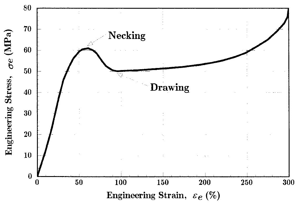
Figure 6: Stress-strain curve for polyamide (nylon) thermoplastic.
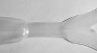
Figure 7: Necking and drawing in a 6-pack holder.
This is called the “true” or “logarithmic” strain.
|
(5) |
|---|
The ratio L/L0 is the extension ratio, denoted as λ. Using these relations, it is easy to develop relations between true and engineering measures of tensile stress and strain (see Prob. 2):
| L | A0 |
→ ϵt = lnL |
(7) | |
|---|---|---|---|---|
| L0 |

6
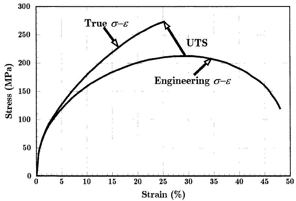
Figure 9: Power-law representation of the plastic stress-strain relation for copper.
A graphical method known as the “Consid`ere construction” uses a form of the true stress-strain curve to quantify the differences in necking and drawing from material to material. This method replots the tensile stress-strain curve with true stress σt as the ordinate and extension ratio λ = L/L0 as the abscissa. From Eqn. 6, the engineering stress σe corresponding to any
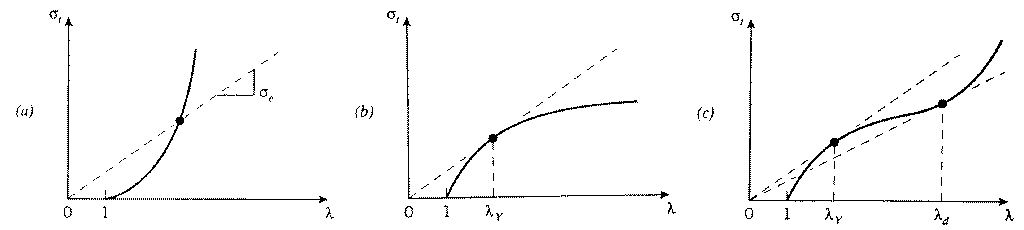
Figure 10: Consid`ere construction. (a) True stress-strain curve with no tangents - no necking or drawing. (b) One tangent - necking but not drawing. (c) Two tangents - necking and drawing.
The increase in strain hardening rate needed to sustain the drawing process in semicrys-talline polymers arises from a dramatic transformation in the material’s microstructure. These materials are initially “spherulitic,” containing flat lamellar crystalline plates, perhaps 10 nm
8
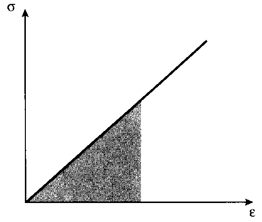
In the absence of molecular slip and other mechanisms for energy dissipation, this mechanical energy is stored reversibly within the material as strain energy. When the stresses are low enough that the material remains in the elastic range, the strain energy is just the triangular area in Fig. 11:
9
| Maximum | Maximum | Modulus of | Density | Max. Energy | |
|---|---|---|---|---|---|
| Strain, % | Stress, MPa | Toughness, MJ/m3 | kg/m3 | J/kg |

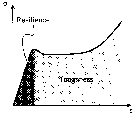
Materials showing good impact resistance are generally those with high moduli of toughness.

absorbed by the material. Conversely, the area under the unloading curve is the energy released
by the material. In the elastic range, these areas are equal and no net energy is absorbed. But
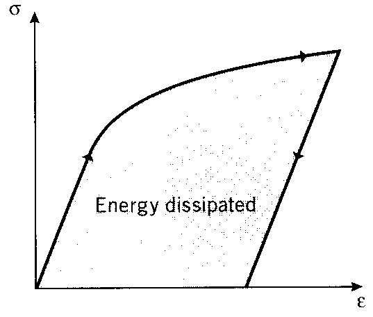
Figure 14: Energy loss = area under stress-strain loop.
There are some practical difficulties in performing stress-strain tests in compression. If excessively large loads are mistakenly applied in a tensile test, perhaps by wrong settings on the testing machine, the specimen simply breaks and the test must be repeated with a new specimen. But in compression, a mistake can easily damage the load cell or other sensitive components, since even after specimen failure the loads are not necessarily relieved.
Specimens loaded cyclically so as to alternate between tension and compression can exhibit hysteresis loops if the loads are high enough to induce plastic flow (stresses above the yield stress). The enclosed area in the loop seen in Fig. 16 is the strain energy per unit volume released as heat in each loading cycle. This is the well-known tendency of a wire that is being
Specimen failure by cracking is inhibited in compression, since cracks will be closed up rather than opened by the stress state. A number of important materials are much stronger in com-pression than in tension for this reason. Concrete, for example, has good compressive strength and so finds extensive use in construction in which the dominant stresses are compressive. But it has essentially no strength in tension, as cracks in sidewalks and building foundations attest: tensile stresses appear as these structures settle, and cracks begin at very low tensile strain in unreinforced concrete.
References
1. The figure below shows the engineering stress-strain curve for pure polycrystalline alu-minum; the numerical data for this figure are in the file aluminum.txt, which can be imported into a spreadsheet or other analysis software. For this material, determine (a) Young’s modulus, (b) the 0.2% offset yield strength, (c) the Ultimate Tensile Strength (UTS), (d) the modulus of resilience, and (e) the modulus of toughness.
2. Develop the relations given in Eqn. 6:
Prob. 1
3. Using the relations of Eqn. 6, plot the true stress-strain curve for aluminum (using data from Prob.1) up to the strain of neck formation.
8. Elastomers (rubber) have stress-strain relations of the form
|
� |
|---|
Use the Consid`ere construction to show whether this
9. Show that a power-law material (one obeying Eqn. 8) necks when the true strain ϵt becomes equal to the strain-hardening exponent n.
values of stress and strain, with equal result.� σ dϵ can be computed using either engineering or true
13


