

The inverse matrix times the matrix produces the identity matrix
Direction Cosine Matrix IMU: Theory
William Premerlani and Paul Bizard
|
1 | Draft: 5/17/2009 |
|---|
pitch control, and this issue prevented the use of pitch stabilization during a hand launch.
1. The gyros are used as the primary source of orientation information. We integrate the nonlinear differential kinematic equation that relates the time rate of change in the orientation of the aircraft to its rotation rate, and its present orientation. This is done at a high rate, (40 to 50 Hz) often enough to give the servos fresh information for each and every PWM pulse that is sent to the servos.
| [XYZGyros] | DriftAdjustment | W |
|
[RMatrix] |
|---|---|---|---|---|
| Gyros | Orientation |
Kinematics
&Normalization
No doubt you are wondering what a rotation group is, and why it should be respected. You also might be wondering how you can use DCM for control and navigation. You also might have the same questions that UFO-MAN asked on the subject after he read Mahoney’s paper, so we will start with those questions:
• What is a quaternion and why do we use that instead of vector notation?
• Can you briefly explain kinematics in this rotation matrix context?
• Can you briefly explain dynamics in this rotation matrix context?
| 3 | Draft: 5/17/2009 |
|---|
y’ |
|---|
x’
x
|
4 | Draft: 5/17/2009 |
|---|
By matrix composition we simply mean multiplying two rotation matrices together. It can be shown that the resulting matrix represents the net rotation that results from applying the two rotations in sequence that each of the matrices represents.
However, numerical integration introduces numerical errors, and does not produce the same result that symbolic integration. An exact symbolic integration of the exact gyro signals will produce the exactly correct rotation matrix. Numerical integration, even if we had the exact gyro signals, will introduce two sorts of numerical errors:
error, starting at the analog to digital converter, and building
whenever you perform a calculation that does not preserve all of the bits of the result.One of the key properties of the rotation matrix is its orthogonality, which means that if two vectors are perpendicular in one frame of reference, they are perpendicular in every frame of reference. Also, that the length of a vector is the same in every frame of reference. Numerical errors can violate this property. For example, since the rows and columns are supposed to
represent unit vectors, their magnitude should be equal to one, but numerical errors could cause them to get smaller or larger. Eventually they could shrink to zero, or go to infinity. The rows and columns are supposed to be
perpendicular to each other, numerical errors could cause them to "lean" into each other, as shown below:
| ||xb|| = 1 | xb yb zb |
|---|
An antisymmetric matrix is a matrix in which each element in the matrix is equal to the negative of the element with swapped row and column index. So, for example, if the element in the first row, third column is 0.5, then the
|
6 | Draft: 5/17/2009 |
|---|
-b -c 0
In our case, kinematics is concerned with the implications of rigid body rotation. It results in a nonlinear differential equation that describes the time evolution of the orientation of the body in terms of its vector rotation rate. The direction cosine matrix is all about kinematics.
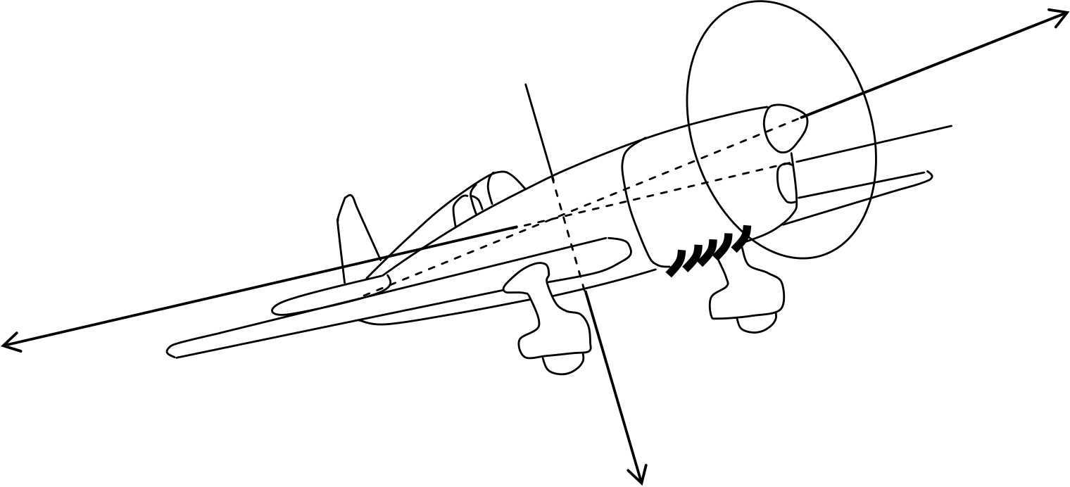
2. To control the roll of an aircraft, you need to know the bank attitude of the aircraft, which you can find by taking the dot product of the pitch axis of the aircraft with the ground vertical.
3. To navigate, you need to know the yaw attitude of the aircraft with respect to the direction that you want to go, which you can find by taking the cross product of the roll axis of the aircraft with a vector in the direction that you want to go. This works even if you are upside down. To find out if your aircraft might be pointing in the opposite
5. To find out the turning rate of the aircraft around the vertical earth axis, transform the gyro rotation vector to the earth frame of reference, and take the dot product with the vertical axis.
We now get deeper into the details of the theory.
| θ | ψ | ye | φ |
|
|---|
xe
|
8 | Draft: 5/17/2009 |
|---|
xb
yb
| R | sin | φ sin | θ cos ψ | − | cos sin ψ |
|
||||||
|---|---|---|---|---|---|---|---|---|---|---|---|---|
|
||||||||||||
| sin | φ sin | θ sin ψ | + | cos cos ψ | ||||||||
| − | sin |
|
sin | |||||||||
of a square matrix, if it exists, is indicated as R−. The inverse of a matrix times the matrix produces the identity matrix. (The identity matrix has all ones on the diagonal, and all zeros everywhere else. Multiplying any matrix by the identity matrix leaves it unchanged. In the case of rotation matrices, it turns out that the transpose of the R matrix is equal to its inverse:
|
10 | Draft: 5/17/2009 |
|---|
| RR | T | = | R R T | = | I | = | 1
|
0 | 0 | Eqn. 5 | |
|---|---|---|---|---|---|---|---|---|---|---|---|
| 1 | 0 | ||||||||||
| 0 | 1 |
A very useful property of the rotation matrix is that we can compose
rotations. We can multiply several rotations matrices together, and get a rotation matrix that is equivalent to applying all of the rotations in succession. We have to be careful to apply the rotations in succession on the left side of what we already have. For example, if we have three rotation matrices, from orientation A to orientation B, from B to C, and from C to D, we can compute the rotation matrix that will go from orientation A to orientation D according to:
The reason that we have to be careful about the sequence of operations when multiplying rotations matrices is that matrix multiplication is NOT commutative. That is, the order of matrix multiplication matters very much..
This is consistent with rotations, which are not commutative either. For example, consider what happens if a plane pitches around its own pitch and roll axes by 90 degrees each. The order very much matters. Suppose that is pitches up by 90 degrees, followed by a roll of 90 degrees. At that point the plane will be traveling vertically. However, if it rolls first, and then banks, it will be traveling in the horizontal plane.
| 11 | Draft: 5/17/2009 |
|---|
Two very useful vector products that we will use in computing DCM and in using its elements for navigation and control are the dot product and the cross product. The dot product of two vectors A and B, is a scalar computed by performing a matrix multiplication of a A as a row vector with B as a column vector producing:
| A | ⋅ | B | = | A B T | = |
|
A y | A z | ] | B | x | = | A x | B | x | + | A B y | y | + | A B z | Eqn. 8 | |||
|---|---|---|---|---|---|---|---|---|---|---|---|---|---|---|---|---|---|---|---|---|---|---|---|---|
| B | y | |||||||||||||||||||||||
| B | z |
| ( A | × | B | = | A y | B | z | − | A B z |
|
Eqn. 10 | |
|---|---|---|---|---|---|---|---|---|---|---|---|
| ( A | × | B | = | − | |||||||
| A z | B | x | A B x |
|
|||||||
| ( A | × | B | = | − | |||||||
| A x | B | y | A B y |
w
v
| k |
|---|
k : unit vector orthogonal to the plane defined by u and v
Stated another way:
With the preliminaries out of the way, we now move on to the central concept of the DCM algorithm: the nonlinear differential equation that relates the time rate of change of the direction cosines to the gyro signals. Our goal is to compute the direction cosines without making any approximations that violate the nonlinearity of the equations. For the moment, we assume that the gyro signals have no errors. Later on we will address the issue of gyro drift.
Unlike rotating mechanical gyros, which stay fixed in space while the aircraft rotates around them, electronic rate gyros rotate with the aircraft, producing signals proportional to the rotation rate. Since rotations do not commute, and the sequence of rotations matter, we cannot get by with simply integrating the gyro rate signals to get angles, that will not work. What we have to do is look to the kinematics of rotations to see what we need to do to get the correct answer.
| Eqn. 12 |
|---|
We make the following observations:
| r | ( ) | = | t r ( ) +∫d θ |
( ) | × | r | Eqn. 13 | |||||||
|---|---|---|---|---|---|---|---|---|---|---|---|---|---|---|
| d θ | ( ) | |||||||||||||
| r | ( ) | |||||||||||||
|
d θ | ( ) | × | r | ( ) | = |
|
|||||||
The vectors in equation 14 are the rows of the R matrix in equation 1. The next question is how to conveniently implement equation 14. We take the same matrix approach that Mahoney [1] uses. We start by going back to the differential form of equation 14:
| ( ) | + | r earth | ( ) | × | d θ | Eqn. 15 |
|---|
compensation feedback controller to the measurement that the gyros make, to produce our best estimate of the true rotation rate:
| ω | Eqn. 16 | |
|---|---|---|
| ω | ||
| ω |
Basically, the GPS and accelerometer reference vectors that we have are used to compute a rotational error, which is fed into the computation through the feedback controller, and back into the rotation update equation via equation Eqn. 16.
When we repeat equation 14 for each of the earth axes, we can put the result into a convenient matrix form:
Equation 17 is a recipe for updating the direction cosine matrix from gyro signals. It is equivalent to Manhoney’s result. The values of 1 on the diagonal of the matrix in equation 17 represent the first term in equation 15. The smaller, off-diagonal elements represent the second term in equation 15.
| 15 | Draft: 5/17/2009 |
|---|
numerical round-off and gyro drift, offset, and gain errors. In the next two sections we will explain how to cancel the errors.
Renormalization
We apportion half of the error each to the X and Y rows, and approximately rotate the X and Y rows in the opposite direction by cross coupling:
| Eqn. 19 |
|---|
You can verify that the orthogonality error is greatly reduced by substituting equation 19 into 18, keeping in mind that the magnitude of each row and column of the R matrix is approximately equal to one. Apportioning the error equally to each vector yields a lower residual error after the correction than if the error were assigned entirely to one of the vectors.
The next step is to adjust the Z row of the matrix to be orthogonal to the X and Y row. The way we do that is to simply set the Z row to be the cross product of the X and Y rows:
| Eqn. 20 |
|---|
What equation 21 says to do to adjust the magnitude of each row vector to one, is to subtract the dot product of the vector with itself (the square of the magnitude), subtract from three, multiply by ½, and multiply each element of the vector by the result.
2. Feed the rotation error vector back through a proportional plus integral (PI) feedback controller to produce a rotation rate adjustment for the gyros. (A PI regulator is a special case of a commonly used feedback regulator called a PID regulator. The D stands for derivative. In our case, we do not need the derivative term.)
3. Add (or subtract, depending on your sign convention for the rotation error) the output of the PI controller to the actual gyro signals.
| 17 | Draft: 5/17/2009 |
|---|
We use accelerometers to provide a reference vector for the Z axis of the airplane. Details will be given in a separate section. We use the GPS as a reference for the horizontal projection of the X axis (roll axis) of the plane. Our two reference vectors happen to be perpendicular to each other. That is convenient, but not absolutely necessary.
For either of the two reference vectors, the orientation error is detected by taking the cross product of the measured vector with the vector that is estimated by the direction cosine matrix. The cross product is particularly appropriate for two reasons. Its magnitude is proportional to the sine of the angle between the two vectors, and its direction is perpendicular to both of them. So it represents an axis of rotation, and an amount of rotation, that would be needed to rotate the measured vector to become parallel to the estimated vector. In other words, it is equal to the negative of the orientation rotational error. By feeding it back to the gyros through the PI controller, the estimated orientation is gradually forced to track the reference vectors, and gyro drift is cancelled.
We will now get into more detail for the two references that we are using.
There are two different coordinate systems for GPS units to report location and velocity. One system reports longitude, latitude, altitude, velocity over ground, and course over ground. Course over ground is the angle of the course measured clockwise from the north. Interestingly enough, this is the same angle as measured in the mathematical sense (counter clockwise) around the Z axis in the body reference frame of the plane, with the Z axis pointing down. In this system, vertical velocity is available through the binary interface.
The other system, ECEF (earth-centered, earth-fixed), reports X, Y, Z position and velocity, with the origin of the right-handed X, Y, Z coordinate system at the center of the earth.
| 19 | Draft: 5/17/2009 |
|---|
1. Reporting latency. Under certain circumstances, for some GPS units it may take as long as 12 seconds for the computed data to be
transmitted.2. Filtering. All GPS units perform some sort of filtering to improve the accuracy of position and velocity estimation. This will result in a smoothing effect on the data when the GPS changes its velocity or position, so that the new information is not seen instantly, but rather becomes apparent gradually.
In addition to a simple latency, you will generally also run into a delay caused by internal filtering done by the GPS. All GPS units perform some sort of filtering of the data by the very nature of how they do their computations.
There is an inherent compromise in any system between accuracy and transient response. The more accurate you want to know something, the longer it will take to estimate it. In most units, the filtering shows up as a smoothing of the data. Typically, the dynamic response of many types of GPS is a simple exponential response with a 1 second time constant, so that it takes about 3 seconds to fully respond to a step change. If you ignore the GPS dynamics, there will be a small error introduced into your navigation calculations during a turn. One of us (Paul) saw that it is possible to
compensate for this small error by introducing a filter between the direction cosine matrix and the input to the yaw drift correction. [Do we need a figure?].


