
The block diagram flow chart shown fig
| ARTICLE IN PRESS |
|---|
Atmospheric Research xxx (2008) xxx–xxx
 |
Contents lists available at |  |
|---|---|---|
| Atmospheric Research | ||
| journal homepage: www.elsevier.com/locate/atmos |
| 1. Introduction | and references cited therein). Bulk aerodynamic method has |
|---|
⁎ Corresponding author. Department of Space, Govt. of India, Indian Space Research Organization, Space Physics Laboratory, Vikram Sarabhai Space Centre, Thiruvananthapuram-695 022 Kerala, India. Tel.: +91 9895656150; fax: +91 471 2706535.
E-mail address: (D.B. Subrahamanyam).
ARTICLE IN PRESS 2 D.B. Subrahamanyam et al. / Atmospheric Research xxx (2008) xxx–xxx
Table 1
Details of KMA Oceanic Buoys deployed in the Yellow Sea, Korea Strait
AND EAST SEA
| SI. | Geographical location |
|
Measurement | Distance from main land | Manufacturer | ||
|---|---|---|---|---|---|---|---|
| no. |
|
|
|||||
| 1. | 22101/3 m Discus | Yellow Sea/30-m | Jul. 1996 to Dec. 2001 | 15 km west of Dukjukdo | Coastal (USA) |
| 4. | 34°00′ N, 127°30′ E | 22104/3m Discus |
|
|
16 km east of Keojedo | ||
|---|---|---|---|---|---|---|---|
2. Bulk aerodynamic algorithm
The bulk aerodynamic method estimates the turbulent exchanges of downward momentum flux or stress (MF, τ) in Nm−2, and Sensible Heat Flux (SHF, HS) and Latent Heat Flux (LHF, HL) in Wm−2. This method has been widely used throughout the marine and air–sea interaction studies for more than four decades now. Computation of the surface layer fluxes using this method requires determination of the exchange coefficients for momentum, heat and moisture. In the recent past, there has been significant progress for attaining higher accuracy in estimation of
|
=lnz� | −Wm |
|
2a | |||
|---|---|---|---|---|---|---|---|
| ðÞ | |||||||
| In the present analysis, air–sea interface fluxes are |
|
−Wt | � | ð2bÞ | |||
|
|||||||
| −Wq | � | ð2cÞ | |||||
|
|||||||
|
|||||||
summarized below in this section. Estimation of surface layer 2.3. Estimation of stability parameter (z/L)
turbulent fluxes of momentum, heat and moisture over the
| L ¼ | Tv � u2 k � g � θv4 |
ð3Þ |
|---|
Depending on the magnitudes of stability parameter ‘z/L’, the entire oceanic buoy data is categorized into three classes:
• Unstable conditions: z/Lb0
• Neutral conditions: z/L=0
• Stable conditions: z/LN0.
|
|---|
ARTICLE IN PRESS
D.B. Subrahamanyam et al. / Atmospheric Research xxx (2008) xxx–xxx 5
over the EAMS region and compared the monthly mean of the fluxes with the climatology data. In the atmospheric boundary layer, eddy correlation method is considered as the most direct and reliable method for estimation of surface layer turbulent fluxes of momentum, heat and moisture. However, adoption of this method requires accurate mea-surements of temperature, humidity, horizontal and vertical winds at a high frequency. Due to lack of stable platforms over the oceanic surface, majority of air–sea interface flux estimations are dependent on bulk aerodynamic algorithms. In order to assess the performance of SR algorithm over the EAMS, we compare our estimates of the fluxes with the
|
1 4: |
prescribed climatology for the concerned region. | |
|---|---|---|---|
| ¼ | 3.1. Air–sea interface flux climatology over the EAMS |
With the estimates of friction velocity (u⁎) obtained from Eq. (2a), we follow the empirical relation for roughness length suggested by Charnock (1955). The roughness length (z0) is represented as the sum of two terms — one due to Charnock (1955) (z0c=α·u⁎2/g) and the other is the viscous term (z0s=β·υ/ α·u⁎) due to Smith (1988):
For the Yellow Sea, we make use of the climatology obtained from 1°×1° COADS (Comprehensive Ocean–Atmosphere Data Set) for a period of about 44 years spanning from 1945 to 1989. For comparison of our estimates of SHF and LHF for the Korean Strait and East Sea, we have taken the climatology data suggested by Hirose et al. (1996). In preparation of heat flux climatology over the East Sea, Hirose et al. (1996) made use of four datasets, viz.: COADS, NODC (National Oceanographic Data
where α is the Charnock “constant”. In the present analysis, the values of α and β are taken as 0.011 and 0.11 (after Smith, 1988). The term υ (=14×10−6m2s−1) represents the dynamic viscosity of air. Since it is verified both experimentally and theoretically that the surface drift velocity is approximatelyequal tou⁎ (e.g., Lo, 1993) estimated value of u⁎ is substituted in place of drift velocity (US) for the ensuing iterations in the SR algorithm in Eq. (2a). Based on the above set of equations, the iteration is repeated between Eqs. (1a), (1b) and (5) until theu⁎,θ⁎,q⁎ andz0 calculated from two consecutive iterations converge.
2.6. Estimation of surface layer turbulent fluxes of momentum, heat and moisture (τ, HS and HL)
3. Assessment of SR algorithm over the East Asian Marginal Seas
Based on SR algorithm, Subrahamanyam et al. (2007) have described the seasonal variation of air–sea interface fluxes
ARTICLE IN PRESS 6 D.B. Subrahamanyam et al. / Atmospheric Research xxx (2008) xxx–xxx
region for about five and half years, now we study the impact of wind speed and atmospheric stability on the air–sea interaction parameters over the study domain.
4. Results and discussion
Fig. 4. Comparison of (a) Sensible Heat Flux and (b) Latent Heat Flux for all the five KMA buoys grouped together with the climatology.
4.1. Wind speed dependence of air–sea interface fluxes
4.3. Correlation of air–sea interface fluxes with WS and SST–AT
It is remarkable that, in the recent past also several investigators have shown a high degree of correlation be-tween the LHF and WS, whereas such a correlation was not seen for SHF and WS. In our present analysis, segregation of the entire data into three categories of unstable, neutral and stable conditions gave us an opportunity to investigate the probable reasons for differences in correlations of SHF and LHF with the varying wind speeds. For this, we draw a set of histograms showing the correlation coefficients between the air–sea interface fluxes and WS and also for DT (=SST–AT) for different stability conditions (Fig. 6). Correlation coefficient between SHF and WS is denoted as r(WS, SHF) and so on for
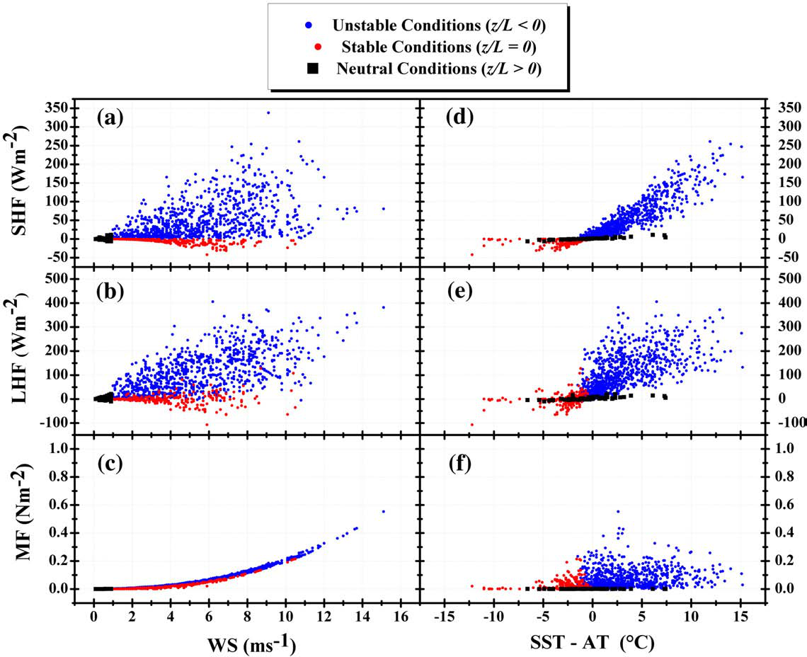
Fig. 5. Left panel: Wind speed dependence of (a) Sensible Heat Flux; (b) Latent Heat Flux; (c) Momentum Flux and Right Panel: SST–AT dependence of (d) Sensible
r(WS, SHF) values show positive correlation for the unstable (~53%) and neutral conditions (~10%), whereas it shows a
negative correlation (~−61%) for stable conditions. In contrast
of MF, irrespective of the stability conditions, it always shows
a steady and good correlation with the WS and r(WS, MF) are always higher than 82% (Fig. 6a). For unstable and stable
▪ SHF Variations: SHF show good correlation with the SST–AT variations, while its WS dependence is poorly defined. For unstable conditions, SHF yields positive correlation with the WS, whereas it shows a negative correlation with WS for stable conditions.
▪ LHF Variations: LHF show a positive correlation with the WS as well as SST–AT, however such a positive correlation is more prominent for SST–AT. On one hand, where LHF yields good correlation with WS for unstable conditions, it does not show clear WS dependence for neutral and stable
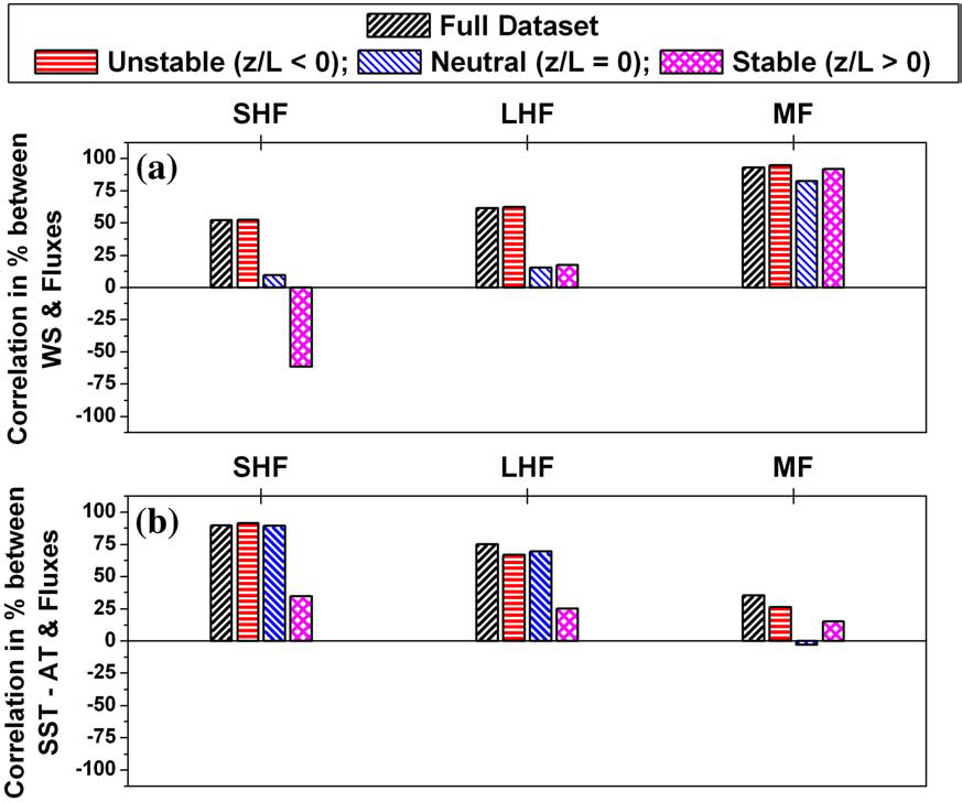
Fig. 6. Histograms of correlation coefficients of Sensible Heat Flux (SHF), Latent Heat Flux (LHF) and Momentum Flux (MF) with (a) Wind Speed and (b) SST–AT for varying stability conditions.
| SI. | Flux |
|
Correlation coefficient in (%) | |||
|---|---|---|---|---|---|---|
| no. |
|
Unstable | Full | |||
| conditions | conditions | conditions | data | |||
| 1. | SHF |
|
|
52.10 | ||
| 2. | LHF | 89.82 | ||||
|
|
61.78 | ||||
| 3. | MF | 66.91 |
|
75.13 | ||
|
93.24 | |||||
|
|
35.58 | ||||
Chu, P., Yuchun, C., Kuninaka, A., 2005. Seasonal variability of the Yellow Sea/East China Sea surface fluxes and thermohaline structure. Advances in Atmospheric Sciences 22, 1–20.
DeCosmo, J., Kastaros, K.V., Smith, S.D., Anderson, R.J., Oost, W.J., Bumke, K., Chadwick, H., 1996. Air–sea exchange of water vapor and sensible heat: the Humidity Exchange Over the Sea (HEXOS) results. Journal of Geophysical Research 101, 12001–12016.
ARTICLE IN PRESS 10 D.B. Subrahamanyam et al. / Atmospheric Research xxx (2008) xxx–xxx
Kraus, E., Businger, J.A., 1994. Atmosphere–Ocean Interaction. Oxford University Press, New York. 362 pp.
Subrahamanyam, D.B., Radhika, R., 2003a. Structural characteristics of marine atmospheric boundary layer and its associated dynamics over the Central Arabian Sea during INDOEX, IFP-99 Campaign. Current Science 85 (9), 1334–1340.
Subrahamanyam, D.B., Radhika, R., 2003b. Wind Speed dependence of air–sea exchange parametersover theIndian Ocean during INDOEX,IFP-99. Annales Geophysicae 21/7, 1667–1679.
Intercomparison of air–sea interface fluxes over the Yellow Sea and Korea Strait — impact of tsushima warm current. Boundary Layer Meteorology 127, 333–344.
WCRP-112, 2000, Intercomparison and Validation of Ocean–Atmosphere Energy Flux Fields (Final Report of the Joint WCRP/SCOR Working Group on Air–Sea Fluxes: WMO/TD-No. 1036).


