

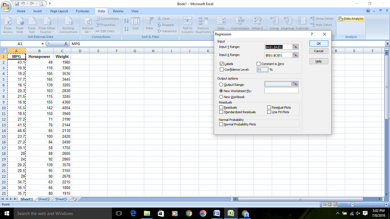
Select the option labels and set the confidence level
14.5
Step 1: Copy the data from the word file and paste it into an Excel worksheet.
b2 = Weight
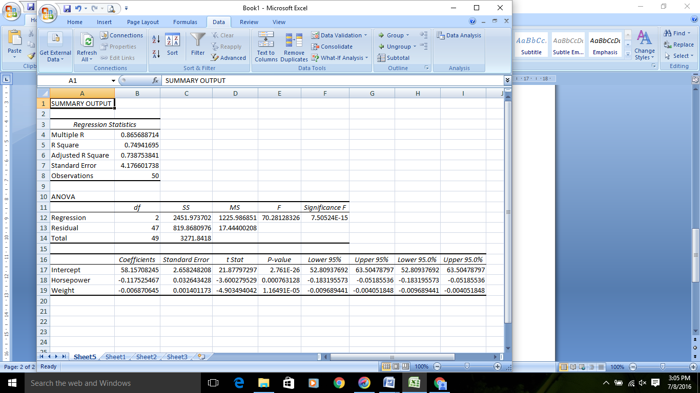
The slope b1 shows that with an increase of 1 horsepower in the engine, the mileage of the car decreases by 0.11 miles per gallon and vice versa.
b2 = 2000
Hence, the miles per gallon (MPG) will be:
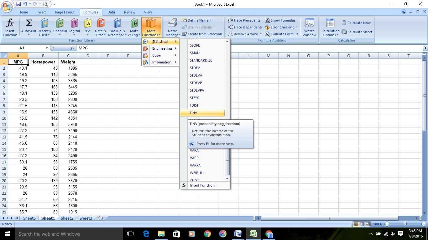
To calculatetα/2, select the TINV function in Excel (Formulas -> More Functions -> Statistical -> TINV)
Confidence interval = 37.56 ± (2.009*4.176) = (29.17, 45.95)
The prediction interval will be:
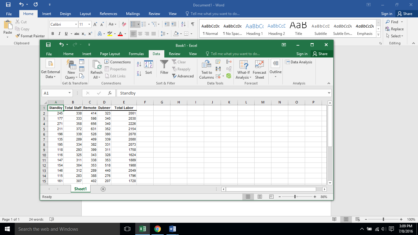
Step 1
Copy data on to an excel sheet.
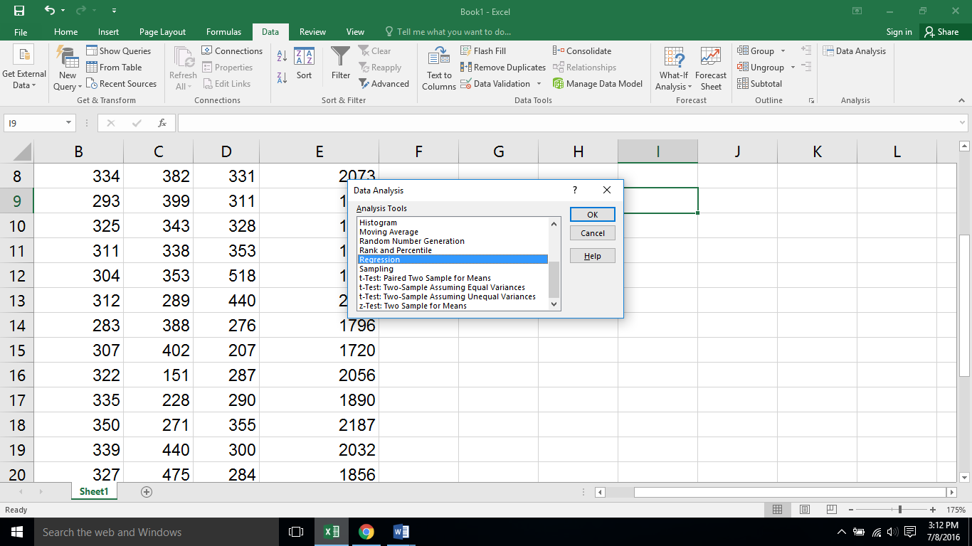
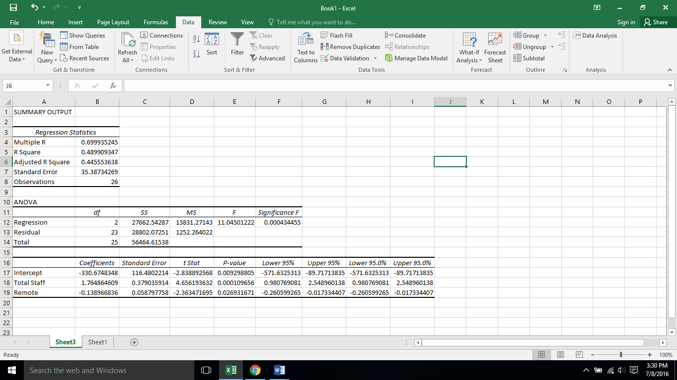
Now answer the question using the table:
X1=Total staff present
X2= Remote hours
The slope b2 means that if 1 unit of change is seen in remote hours then the standby hours would decrease by 0.13 units.
Thus we can conclude that standby hours are directly proportional to total staff present while remote hours and standby hours are inversely related
=493.6 hours
y=Y$\pm \ t_{\frac{\alpha}{2}}s_{Y}$
= 433.17
y=493.6-(-1.708*35.38)
MSE=1252.26
y=493.6 ± ( − 1.708*$\sqrt{{35.38}^{2} + 1252.26}$
Step 2: To calculatetα/2, use the Excel function TINV.
Go to Formulas -> More Functions -> Statistical -> TINV
Step 3: Use the formula described in Step 1 to get the confidence interval for the population slope.
Confidence interval= 0.79116 ± (2.16*0.06295)
Null hypothesis: H0 : b = 0
Alternate hypothesis: H1 : b ≠ 0
tcal = 12.57 (from the regression results given)
Step 5: Since tcal > critical value, we reject the null hypothesis H0.
Alternate hypothesis: H1 : c ≠ 0
Step 2: t test will be used.
Step 5: Since tcal > critical value, we reject the null hypothesis H0.
Thus, the variable MIDSOLE makes a significant contribution to the model
Step 3
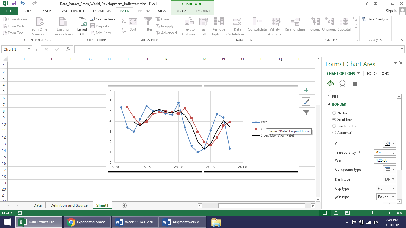
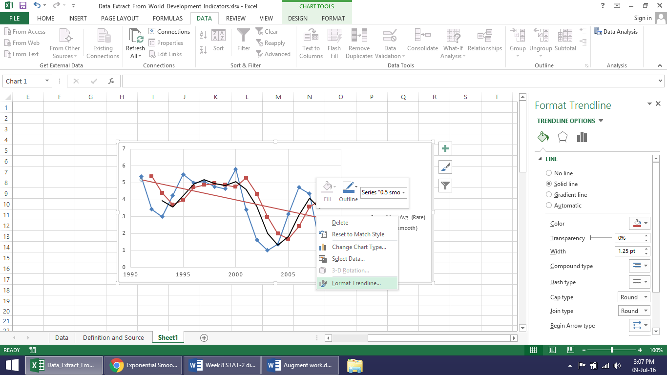
Select points the data points on the graph and right click. Click on the option add trend line. A dialogue box will appear select moving average and change the period to 3. Click ok.
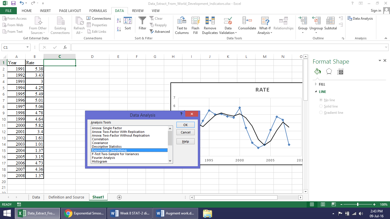
Click on data and select data analysis tool pack. A dialogue box opens. Select exponential smoothening from the dialogue box.
Step 6
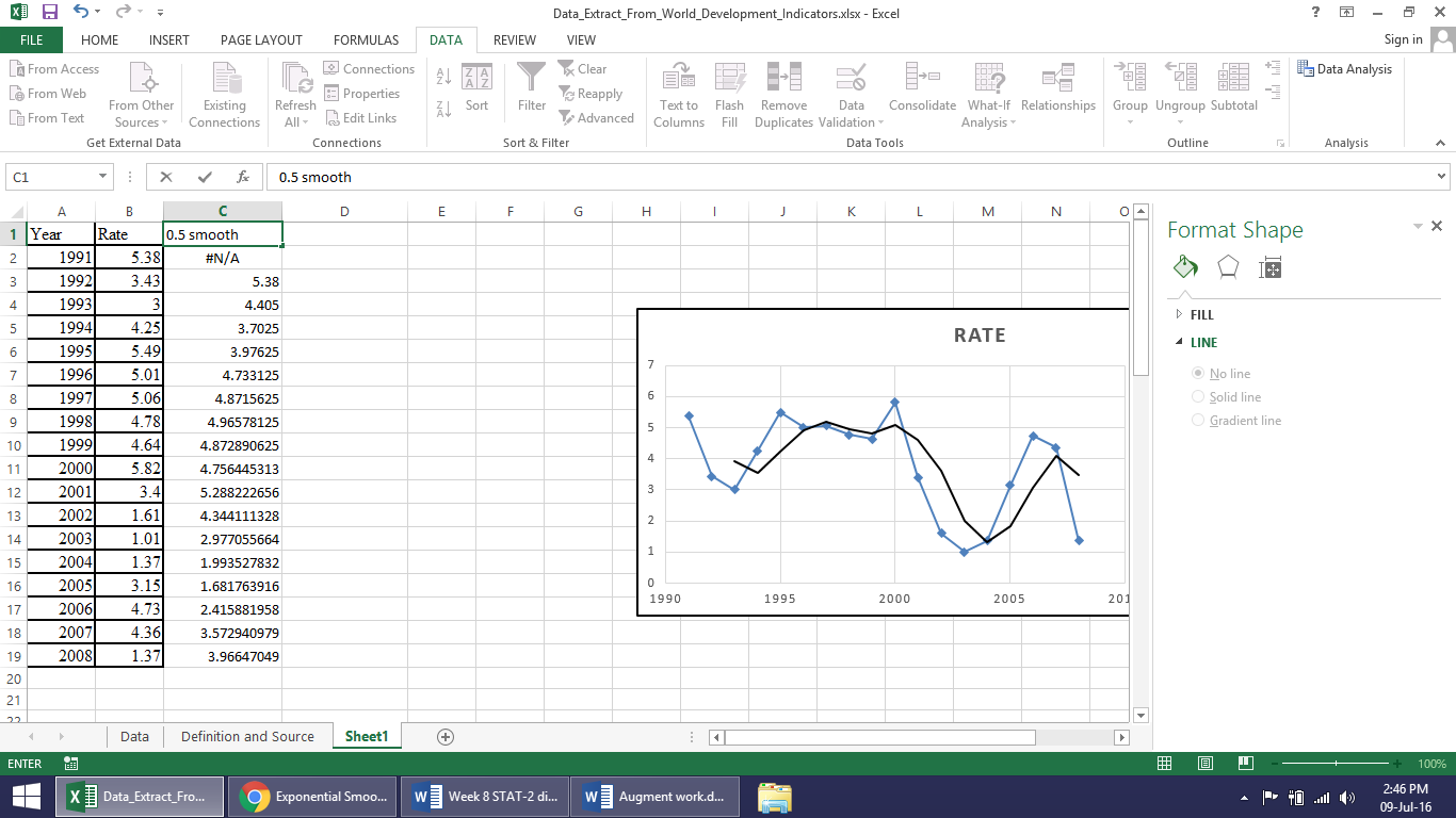
The following graphs appears
= 2.8086
E.
Y = -0.1285x + 5.5173
The forecast for 2009 is
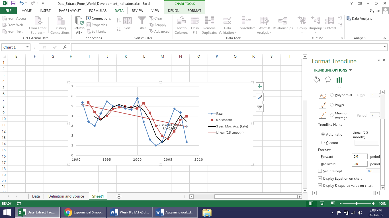
16.13
Find GDP data online
Plot a line graph. Click on insert and select icon of line graph. Select data for y axis from B1 to B30 while for x axis select data from A1 to A30. To plot a trendline select the data points right click and you will find the option of adding a trendline selct the option. Then right click on trendline and select the option of formatting trendline select display equation and R2. Click ok. The graph with all the iformation will be plotted.
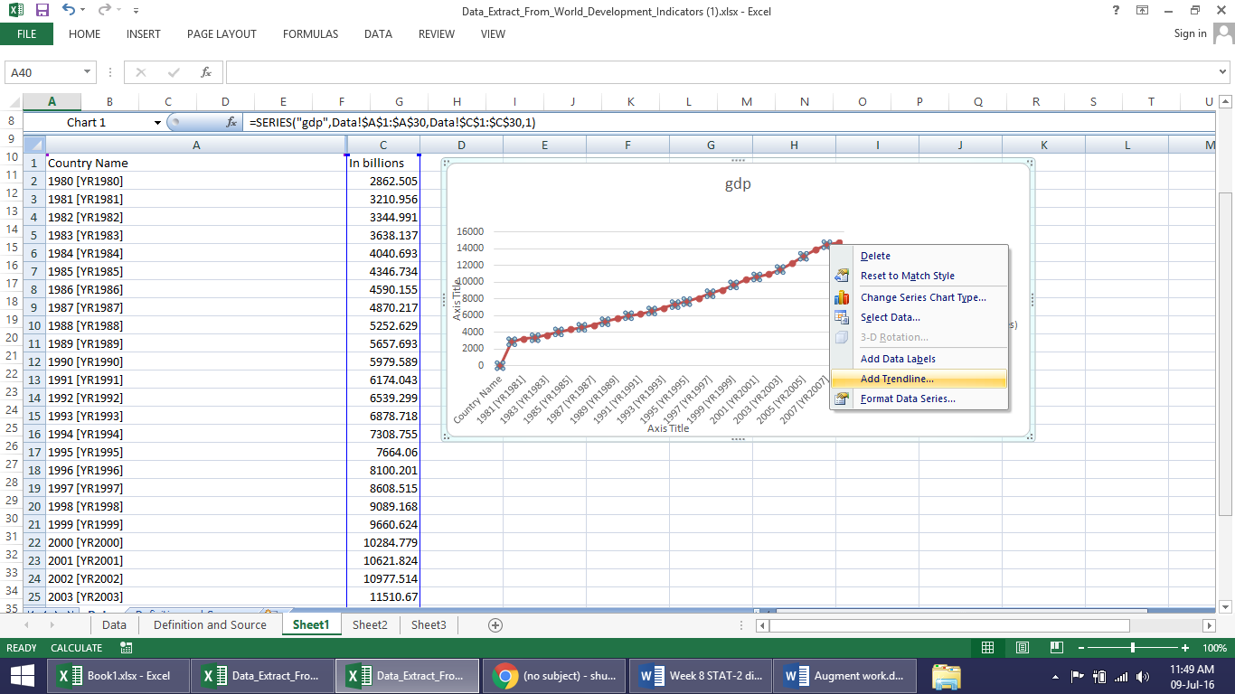
Y=431.34*x+968.61
GDP=431.34*(Year) + 968.61
X=2010 (31st observation)
Y=431.34*(31)+968.61
16.15
16.47
H.
Forecast of March 2009


