
Return the original format use format short using matlab
ECE 350L: Signals and Systems Lab
Fall 2015
Lab 9 Bode Plots & Analog Filter Design
AssignmentDeliverables:
Submit through blackboard a report that includes your completed lab worksheet and all generated Matlab files. Ensure all plots are pasted appropriately into the lab worksheet and answer questions presented. All plots should have descriptive titles (with your initials) and appropriately labeled axes.An ideal (real) low-pass filter has a passband that begins at zero Hertz and extends up to the cutoff frequency. The stopband of the ideal low-pass filter begins at the cutoff frequency and continues up to infinite frequency. The magnitude of the frequency response is equal to one for all frequencies in the passband and equal to zero for all frequencies in the stopband. The equivalent is true for the negative frequencies.
Ideal filters do not exist in the real world. The best we can do is to approximate the ideal filter. A filter with a higher order will always be able to better approximate the ideal filter than a filter with lower order. However, increasing the order of a filter increases its cost and complexity. As a result, we will specify how close to the ideal filter we need to come for some application, then select a filter with the smallest order possible to do the job.
There are several standard classes of filters that have been well analyzed for many years. They differ mostly in how the deviations of the magnitude frequency response behave with respect to the ideal filter. These deviations are referred to as passband ripple and stopband ripple (δ1 and δ2). Butterworth filters have the property that the ripple in the passband is as small as possible. The magnitude of the frequency response of a Butterworth filter falls monotonically as frequency increases. Another class of filters that falls monotonically is the Bessel filter. Other filter classes such as Chebyshev and Elliptical filters are not monotonically decreasing with increasing frequency.
Filter Order
The first thing that you have to do when designing an analog low-pass filter is to determine the minimum order that satisfies your specifications. This is automated in MATLAB. The command buttord finds the lowest order butterworth filter that will do the job. Similarly, ellipord finds the lowest order elliptical filter that will do the job. Chebyshev filters come in two types (Type I and Type II). cheb1ordand cheb2ord finds the lowest order for these filters. There does not appear to be an order selection for Bessel filters in the current version of MATLAB.The coefficients that you find for filters often will show up as 0.0000 in this lab. This is not because the value is actually zero (which MATLAB will print as 0), but because the value is smaller than one half of the least significant digit printed. To see more significant digits, use the command format short g, to return to the original format use format short.
2
1-4)Plot the magnitude of the frequency response of the Butterworth filter that you specified in part 1 using a linear scale. What is the magnitude of the frequency response at 500Hz? What is this magnitude when converted to dB? Does this meet your specs? Is the magnitude of the frequency response ever greater than one?
From this point forward, it will be necessary to pay attention to your variable naming conventions. Be sure not to overwrite your parameter values for the Butterworth filter and subsequent variables, as we will be using these later on. In addition, use the Matlab help utility for each command to verify the syntax and variable, parameter ordering.
The syntax for the cheb1ordcommand is [n,Wp] = cheb1ord(Wp,Ws,Rp,Rs,'s'). The syntax for the cheby1command is[b, a] = cheby1(N, Rp, Wp, ’s’)where Rp and Wp are as defined above. Use Wp returned by the cheb1ord function.
Chebyshev type II filter.
3-1)Plot the magnitude of the frequency responses on linear axes using different color/or symbols for the Butterworth, versus {Elliptical, Chebyshev type I or II} filters on the same axes.
Additionally, look in MATLAB help file on how to add a legend to the plot. Add a legend with appropriate information. Use the same frequency range. You can plot multiple plots to one plot window using the holdcommand.To begin holding plots type hold on. Type hold off when you are finished plotting to that window.
Part 4 - Second Order Sections & Physical Filter Circuit Design
Filters of order one and two are well understood and can easily be built with op-amps (operational amplifiers), resistors, and capacitors. Filters of order three or more get very complicated. Luckily, filters of order three or more can be broken down into a series of first and second order filters. Building the first and second order filters around op-amps allows us to isolate the components of each filter so that they will not interact with each other. Each filter in such a series is called a “second order section”. In order to build a filter using second order sections, it is necessary to break the differential equation describing the filter into several pieces.A Butterworth filter will only include the input x(t) in its differential equation and none of the derivatives of x(t). For a third order Butterworth filter MATLAB will return something equivalent to the following: b = [0 0 0 1] and a = [a3 a2 a1 1]. MATLAB will actually give you something like b = [0 0 0 g] and a = [ga3 ga2 ga1 g]. While this might seem strange, it is always valid to multiply or divide all of the values in both the a and b vector by the same constant. So, in this case divide both a and b by g.
| xt () | = | + | + | dt |
+ | y t ( ) |
|
(1) |
|---|

Building Second Order Sections
In order to build the filter using second order sections, we need to specify the frequency response as a product of second order frequency responses (one of the responses will be first order if the overall order of the filter is odd). So, for a third order Butterworth filter, we need something that looks like
| H | ( | j ω ) | = | 1 | • | 1 | (3) | ||||||||||||||
|---|---|---|---|---|---|---|---|---|---|---|---|---|---|---|---|---|---|---|---|---|---|
| c 1 | ( | j ω ) | d | 2 | ( | j ω ) | 2 | + | d | 1 | ( | j ω ) | + | 1 | |||||||
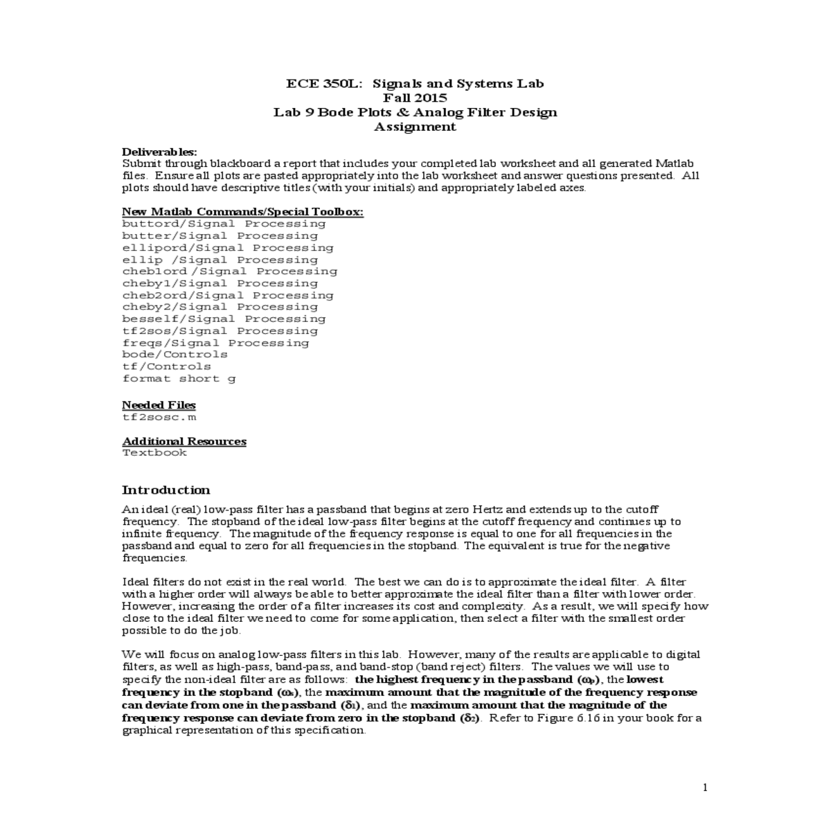
This can be accomplished by finding the roots of the left hand polynomial (numerically), grouping the roots into complex conjugate pairs, and using the conjugate pairs to reform second order polynomials. Luckily, MATLAB has also automated this process. The command tf2sos takes a transfer function form (the one that uses the original b and a matrices) and turns it into a list of second order sections. Unfortunately, the tf2sos command is for digital filters and there does not appear to be an equivalent command for analog filters.
The tf2sos command has been rewritten for you, so that you can use it for analog filters in this lab. The command was renamed tf2sosc. In order to use this command, you must tell MATLAB where to find it. Do this with the command addpath or copy it to your working directory. Be aware, however, that the function tf2sosc is not a standard part of MATLAB and therefore will not work elsewhere, unless you copy it and take it with you. The syntax of the tf2sosc command is [sos, g] = tf2sosc(b, a).
| . |
|---|
Figure 1. The structure of the SOS array.
4-1)Write down the frequency response of the Butterworth filter you are designing in second order section format(i. e., as equations of several first or second order frequency responses multiplied together). Report H(jω) both as a formula and as the returned matrix. Be sure to check the g matrix to see if the gain is equal to one. If it is not exactly one, multiply this gain in front of the series of frequency responses.
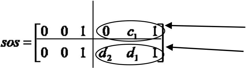
Figure 2.The layout of the second order low-pass filter.
The cutoff frequency of the above filter (frequency where power is one half, or 3 dB down point) is
| ω= | 1 | (5) | |
|---|---|---|---|
| 0 | RC |
damping ratio of 2 . However, second order sections of Butterworth filters are not themselves Butterworth filters, so the damping ratio of each individual second order section must be determined in order to build it. The damping ratio of the above Sallen-Key filter is
ζ = 3 – A . (7)
| Hj ω ) | = | (8) | ||||||||
|---|---|---|---|---|---|---|---|---|---|---|
| 1 ( | j ω ) | 2 | + | ζ | ( | j ω ) 1 + | ||||
|
ω 0 | |||||||||
To make this match the second order section of our third order Butterworth filter example, it is necessary that
| and | (10) |
|---|
This can be solved to get
5-4)If we use a 0.1 μF capacitors in our filters, what value of R should we choose for each second order section in the Butterworth filter?
If we have a filter whose overall order is odd, one of the “second order sections” will actually be first order. We can build a first order low-pass filter using an op-amp, a capacitor, and three resistors as shown in Figure 3.
| C | _ | Rf | Vout |
|---|
Figure 3. The layout of the first order low-pass filter.
The cutoff frequency of this filter is given by
| A | =1+ | R | F | (14) | |
|---|---|---|---|---|---|
| R i | |||||
So, the cutoff frequency and gain are given by the same equations as the second order filter. There is no such thing as a damping ratio for a first order filter. Since there is no damping ratio to control, the gain of the first order filter can be set to whatever one wishes.
|
|
(16) |
|---|
|
Ri1 | C2 | Ri2 |
|---|
Figure 4. The layout of the third order Butterworth filter.


