
Pressure versus rate analysis for the step rate test fig


N
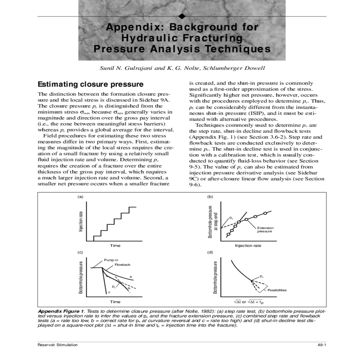
The closure pressure pc is distinguished from the minimum stress σmin because σmin generally varies in magnitude and direction over the gross pay interval (i.e., the zone between meaningful stress barriers) whereas pc provides a global average for the interval.
Field procedures for estimating these two stress measures differ in two primary ways. First, estimat-ing the magnitude of the local stress requires the cre-ation of a small fracture by using a relatively small fluid injection rate and volume. Determining pc
requires the creation of a fracture over the entire thickness of the gross pay interval, which requires a much larger injection rate and volume. Second, a smaller net pressure occurs when a smaller fracture
| (a) | (b) | pc |
|
||
|---|---|---|---|---|---|
| Injection rate |
|
||||
| (c) | (d) | pc | |||
| Bottomhole pressure | Bottomhole pressure | ||||
| Flowback | |||||
| a | |||||
| pc | Possibilities | ||||
|
|
||||
The step rate test is conducted solely to determine pc.
In low-permeability reservoirs, the test generally is performed with completion fluids (e.g., treated
water). The use of polymer fluids may be required in high-permeability reservoirs (Smith, 1985) to control potential fluid loss and ensure fracture creation at lower injection rates.
The y-axis intercept interpretation was used to ana-lyze the step rate test illustrated in Fig. 9-10b. The pressure versus rate plot is entirely characterized by the fracture extension line (Appendix Fig. 3), which has a y-axis intercept of 4375 psi for the estimated value of pc.
An indication of a valid step rate test is that the extrapolated pressure for the zero rate of the line rep-resenting matrix injection should equal approximately the bottomhole pressure preceding the test. The zero-rate pressure is the reservoir pressure, if significant amounts of fluids were not previously injected. This quality control check can also be used while conduct-ing the test when no apparent slope change is
observed for the pressure versus injection rate plot.
| Chapter 9 Appendix: Background for Hydraulic Fracturing Pressure Analysis Techniques |
|---|
Either of the specialized plots, however, may be completely devoid of a significant slope change or may exhibit multiple slope changes. In general, up to six events could be associated with a slope change:
• height recession from the bounding layers
• reservoir radial flow.
Consequently, the shut-in test commonly fails to provide an objective indication of pc and should not be used as the primary procedure for determining it. Experience indicates that the square-root plot may provide a better indication of closure for fluids that do not have effective fluid-loss control from wall-building behavior, whereas the G-plot may provide a better indication for fluids with wall-building behav-ior. The analysis of decline data typically uses both plots to determine the value of pc.
Maintaining a constant flowback rate as the pres-sure decreases is critical for a flowback test. This objective requires a field-rugged, debris-resistant flow regulator that both measures and controls the flow-back rate. The flow regulator should be preset for the desired rate at the pressure expected following the end of injection, and it should be isolated by a closed valve during pumping. Presetting the flow regulator is best achieved by opening it during the last period of the step rate test to establish the desired flowback rate prior to the actual test. The effect of the additional fluid loss can be compensated for by increasing the injection rate. Fluid injection is terminated once the desired constant flowback rate has been attained, and this rate is then maintained throughout the flowback period.
Experience shows that an adjustable choke often plugs because of pipe dope and other debris loosened into the wellbore during the injection period. A gate valve is preferable for controlling the flowback rate. In addition, a pressure sensor and fixed choke at the end of the flowback line can be substituted for a flow meter to reliably measure the flow rate, particularly when the rate is low (i.e., 3 bbl/min or less). Tabu-lated values for the pressure drop versus the flow rate through standard choke sizes are used to select the choke size that will provide the pressure change nec-essary for a reliable pressure measurement at the anticipated flowback rate.
In conclusion, the combination of the upper bound estimate of pc from the intersection of the matrix and fracture extension lines on a step rate test, the lower bound of pc determined from the rebound pressure and the estimate of pc from the y-axis intercept of the fracture extension line as well as the intersection of the two lines during flowback provides multiple, independent values that establish a firm basis for defining pc.
Test sequence
• Residual fluid-loss control from unbroken polymer or additives in the fracturing fluid enables fractur-ing using moderate injection rates with the com-pletion fluid.
• Because the poroelastic effects have stabilized, the step rate/flowback test better replicates the stress conditions that occurred during the preceding cali-bration treatment.
|
Chapter 9 Appendix: Background for Hydraulic Fracturing Pressure Analysis Techniques |
|---|
minimize wellbore expansion effects during pres-sure falloff. For gas reservoirs, this can be achieved by conducting the injection test before a production period. Alternatively, the gas should be circulated from the wellbore or bullheaded into the formation.
– as the stabilized surface pressure measured prior to fluid injection into an overpressured reservoir
– from the surface pressure and hydrostatic col-umn estimated through an accurate measurement of the fluid injected to completely fill the well-bore for an underpressured reservoir
(1)
| A9-5 |
|---|
| q | ( | da t | ) = | 2 | da |
|
(8) | ||||||||||||
|---|---|---|---|---|---|---|---|---|---|---|---|---|---|---|---|---|---|---|---|
| L | t | 1− |
|
( | t | α D | − | ξ | 1 / | α | θ | ||||||||
| p | |||||||||||||||||||
where Af is the fracture surface area at the end of pumping.
The total rate of fluid loss is obtained by the inte-gration of Appendix Eq. 8 over the fracture area:
| ∆t | = | t | − | t | p | = | ∆t | = | t | − | (15) | ||||
|---|---|---|---|---|---|---|---|---|---|---|---|---|---|---|---|
| D | t | p | t | p | |||||||||||
Cumulative fluid-loss volume
The total fluid-loss volume at the end of pumping VLp comprises the cumulative contributions of its CL fluid-loss component VLp,C and spurt VL,S:
| q | ( | A t | )= | 2 | f | f ( | α θ | (11) | V Lp | = | V Lp C | + | (18) | |||||
|---|---|---|---|---|---|---|---|---|---|---|---|---|---|---|---|---|---|---|
| L | f | t |
|
|
||||||||||||||
integrating over the area:
| V L C | = | 2 |
|
αα θ | ) | (13) |
|---|
The functions f(tαD,α,θ) and g(tαD,α,θ) are usually presented in terms of the dimensionless shut-in time
| V Lp C | = | V L C | ( | ∆t | D | = | 0 | ) = | 2 | ( | α θ | ) | (19) |
|---|
Spurt occurs only for wall-building fluids. It ac-counts for the fluid-loss volume prior to the creation of a filter cake and is applicable only during the frac-ture propagation period. Following the spurt period, wall-building fluids exhibit a Newtonian filtrate during the fluid-loss process (i.e., nf = 1 or θ = 1⁄2). The total volume of fluid lost to spurt follows from definition of the spurt coefficient Sp:
|
A9-7 |
|---|
θ = 1⁄2 in Appendix Eq. 41, whereas Appendix Eq. 40 provides the upper bound. An upper bound of unity is assumed because it provides simple, closed-form expressions. The bounding values of α for a wall-building fluid are therefore as in Eq. 9-43:
| V | = | 2 | r | κ C |
|
| α θ | = | 1 | θ | = | 1 | < | α< | 1 | ||||
|---|---|---|---|---|---|---|---|---|---|---|---|---|---|---|---|---|---|---|---|
| Lp | p | L |
|
| 2 |
|
2 |
| V | = | 2 | r C t A g | ( | α θ | θ | ≠ | 1 | (23) | ||
|---|---|---|---|---|---|---|---|---|---|---|---|
| Lp | 2 |
Appendix Eq. 22 is expressed in terms of the spurt factor κ, which provides for the increase in fluid loss over the no-spurt condition:
| g ( | ∆t | D | ) | θ | = | 1 | = |
|
(+ | ∆t | D | ) | −1 2 | + | ∆t | (28) | ||||||||||||||
|---|---|---|---|---|---|---|---|---|---|---|---|---|---|---|---|---|---|---|---|---|---|---|---|---|---|---|---|---|---|---|
| α | = | 1 | ||||||||||||||||||||||||||||
| 2 | ||||||||||||||||||||||||||||||
| ∆t | 3 2 | ) | ||||||||||||||||||||||||||||
| α | 1 | |||||||||||||||||||||||||||||
| 2 | − | = | ||||||||||||||||||||||||||||
| (29) | ||||||||||||||||||||||||||||||
An expression for VLs(∆t) results from subtracting Appendix Eq. 19 from Appendix Eq. 13:
| V Ls | ( | ∆t | ) = | 2 |  tA tA |
= | 1 | − | g | | α θ | = | 1 | | | θ | = | ||||||
|---|---|---|---|---|---|---|---|---|---|---|---|---|---|---|---|---|---|---|---|---|---|---|---|
| ⋅ | | g | | ∆t | , , α θ | ||||||||||||||||||
| | | D | 2 | | 0 | | 2 | | | ||||||||||||||
(26)
| V | ( | ∆t | ) = | 2 | r C t A g ( | ∆t | , , α θ | ) − | g |
|
) ) | θ | ≠ | 1 | ||
|---|---|---|---|---|---|---|---|---|---|---|---|---|---|---|---|---|
| Ls | D | 0 | 2 |
Fracturing fluids produce a Newtonian filtrate follow-ing the deposition of a filter cake. For this case, nf = 1, and Appendix Eq. 7 indicates that θ = 1⁄2. Analytical expressions for fluid loss can be derived for bounding values of α. The lower bound value corresponds to negligible efficiency and is obtained by substituting
All these functions are well behaved. Their values at any other value of α can be obtained through simple interpolation between bounding values.
| g0 | ( | α θ | ) = | Γ | θ Γ ( 1 + α + θ ) |
) |
|
(31) |
|---|
respectively) can be obtained for only select values of their arguments that are applicable to specific field applications. The upper bound of α = 1 applies also for θ ≠1⁄2, and the corresponding functions are
| ( | ∆t | α | = | 1 , | θ | ) = | θ 1 1 [ (+ | ∆t | ) − | ∆t | θ | ] | (32) | |||||||||||||||||
|---|---|---|---|---|---|---|---|---|---|---|---|---|---|---|---|---|---|---|---|---|---|---|---|---|---|---|---|---|---|---|
| g ( | ∆t | D | D | D | 1 + | θ | ] . | |||||||||||||||||||||||
| , | α | = | 1 , | θ | ) = | 1 | [ (+ | ∆t |
|
θ | − | ∆t | (33) | |||||||||||||||||
| D | θ (+ | θ | ) | D | D | |||||||||||||||||||||||||
where 〈w—〉 is the fracture width averaged over the fracture area. The bounding expressions for fracture penetration in Eqs. 9-32 through 9-34 are derived by combining Appendix Eqs. 37 and 39 with the fracture width relations in Eq. 9-27, for which the fracture area Af is proportional to the half-length L for the PKN and KGD models and to R2for the radial model. For the common occurrence of Newtonian fracturing fluid filtrate (i.e., θ = 1⁄2):
L∝t 1 2 η→0 PKN L∝t ( 2 n + 2 )
( 2 n + 3 ) η→1
| R | ∝ | t | 1 4 | + | 2 | ) ( ( |
3 | n | + | 6 | ) | η | → | ||||
|---|---|---|---|---|---|---|---|---|---|---|---|---|---|---|---|---|---|
| R | t | ( 2 | n |
|
|||||||||||||
| ∝ | η | → | |||||||||||||||
Bounding values for fluid efficiencies
| A | = | q t i | η | → | (37) | ||
|---|---|---|---|---|---|---|---|
| f |
|
||||||
| ∝ |
| p net | ∝ | t | 1 4 |
|
η | → |
|
|||||||||
|---|---|---|---|---|---|---|---|---|---|---|---|---|---|---|---|---|
| ∝ | t | 1 2 ( | n + | 3 ) | η | → | ||||||||||
| p net | ||||||||||||||||
| p net | ∝ | t | − | n | /2 | ( + 1 | ) | η | → | |||||||
| p net | ∝ | t | − | n n ( + | 2 | η | → | 1 | ||||||||
|
∝ | t | −3 | n / | 8 | ( + 1 ) | η | → |
|
|||||||
| p net | ||||||||||||||||
| p net | ∝ | t | − | n n ( + | 2 | η | → | |||||||||


| α | 1 | = | 2 | n | + | 2 | ) ( | 2 | n | + | 3 ) |
|
η | → |
|
(40) | |||
|---|---|---|---|---|---|---|---|---|---|---|---|---|---|---|---|---|---|---|---|
| n | + | 1 ) ( | n | + | 2 | ) | |||||||||||||
| 6 | |||||||||||||||||||
| 4 | n | + | 4 | ) ( 3 n | + | Radial | |||||||||||||
For the typical value of θ = 1⁄2, Appendix Eq. 41 shows that α0 = 1⁄2, which is the value used in Eq. 9-43.
Postscreenout pressure relations
| ∆ | w A | fso | = | q i | ∆t | so | − | V Lp | ( | ∆t | so | (42) |
|---|
where ηso is the fluid efficiency at screenout and Viso is the volume injected prior to the screenout.
For an assumed constant injection rate Viso = qitso, Eq. 9-6 and Appendix Eq. 43 can be combined:
| ( | w A | f ) | so | = | η so | q t i so | = | η | so | V Lp | ( ) (− (− |
η so | ) |
|
(44) |
|---|
Because the same set of conditions as that follow-ing the end of injection is assumed to exist following a screenout, the expression for VLp(∆tso) is similar to that in Appendix Eq. 26:
| V Lp | ( | ∆t | so | ) = | 2 |
|
t | p | ( | g ( | ∆t | Dso | ) − | (46) |
|---|
An expression for the treatment efficiency at any time after a screenout η(∆tDso) can be obtained by combining the definition of η from Eq. 9-4 with the width multiplier expression in Appendix Eq. 47:
| η ( | ∆ | ) = − |
|
+( | ∆t | Dso | ) − | g 0 | | (48) | ||||||||
|---|---|---|---|---|---|---|---|---|---|---|---|---|---|---|---|---|---|---|
| Dso | ) | |
κ | so | g 0 | |
| t | so | η so | = |
|
(50) | |||||
|---|---|---|---|---|---|---|---|---|---|---|
| p net so | ||||||||||
| Chapter 9 Appendix: Background for Hydraulic Fracturing Pressure Analysis Techniques |
|---|
Comparison of fixed-length and propagating fractures†
Fracture propagation and closure lead to characteristic pressure and fluid-loss distributions along the inter-face between the fracture and the reservoir. The time history of these distributions establishes the boundary conditions for the reservoir response before and after fracture closure. These conditions are generally dif-ferent from those experienced by fixed-length frac-tures; however, there are also similar conditions that are shared by these two types of fractures. The simi-lar conditions enable applying established fixed-length relations to a propagating fracture. The back-ground for identifying these differences and
similarities is reviewed in this section of the
Appendix to Chapter 9 along with the fixed-length relations that are applicable to the propagating case.Throughout this section, the propagating fracture is assumed to have a rectangular shape (i.e., Af = 2hfL) and a square root of time dependency of the fluid loss (i.e., θ = 1⁄2 in Appendix Eq. 5).
Pressure characterization for a propagating fracture
In general, each of the pressure differences depends on time and position as the fracture propagates and closes.
As shown in Eq. 9-76, ∆pR is represented by the added contributions from the two sources of fluid loss: the pressure difference associated with the CL component of fluid loss ∆pRC and the component associated with spurt loss ∆pRS. Nolte et al. (1997) provided the linear flow expression for ∆pR that includes the time dependence for ∆pRS in Eq. 9-84, which is applicable both before and after closure.
| ∆p | RC | = | ∆p T | ; | ∆p | RS | = | ∆p nf | = | (54) |
|---|
tion pressure during propagation at a constant injec-tion rate. The simultaneous condition of constant pressure and constant rate provides one of the pri-mary distinctions between a propagating and a fixed-length fracture. The fixed-length fracture requires an increasing pressure difference to maintain a constant production rate or a decreasing rate for a constant-pressure condition. From the reservoir perspective, this difference occurs because a propagating fracture has an approximately constant or stationary value of dimensionless time with its associated condition of time invariance for pressure and flow rate.
| T | = p | | 0 5. | η | (55) | |
|---|---|---|---|---|---|---|
| T p | t | |
Appendix Eq. 55 shows that T is stationary and equal to its value at the end of pumping for a fracture with vanishing efficiency (i.e., η → 0). The equation also shows that T retains only a weak dependence on time for moderate values of efficiency. For example, for η = 0.5, T decreases only 19% during the second half of a treatment. Furthermore, Fig. 9-38 shows that a 10-fold change in the dimensionless time is required before any meaningful change occurs in the reservoir flow regime. The reservoir flow regime, therefore, is even more weakly dependent on dimensional time than the case for dimensionless time. It can be con-cluded that typical conditions for fracture propagation result in essentially a stationary dimensionless time and reservoir flow regime.
The approximately stationary value of T provides another primary difference between a propagating fracture and a fixed-length fracture for which dimen-sionless time increases with increasing dimensional time. An additional difference for a calibration treat-ment is that it does not retain fracture conductivity,
However, the fixed-length fractures have different transitional flow behaviors (e.g., Gringarten et al., 1974) and represent the transitional behavior in
Fig. 9-38 with differing degrees of accuracy. The uniform-flux fracture has a deviation of less than 5% from the propagating case for the complete time range shown in the figure (i.e., that applicable to the impulse representation). The transitional behavior for the uniform-pressure case deviates by almost 25% from that for the propagating fracture. The maximum deviation in both cases occurs slightly before the knee time. These quantitative results confirm the cited qualitative inferences from Fig. 9-35, that the after-closure behavior of a propagating fracture can be represented by a uniform-flux fixed-length fracture.
| ∆p | RC | = | C L | (57) | |
|---|---|---|---|---|---|
| ∆p T | C c | ||||
| C c | = |
|
|
(56) |
|---|
| p | D up | ( )= | k | t | p | ∆p | RC | ( ) | η | → | 0 , | κ | → |
|
(60) |
|---|---|---|---|---|---|---|---|---|---|---|---|---|---|---|---|
| ∝ | C L L | ||||||||||||||
An expression for the radial coefficient CR can then be obtained by combining Appendix Eq. 59 with the definitions of dimensionless time (Eq. 9-75), Cc (Appendix Eq. 56) and the pressure ratio (Appendix Eq. 58):
| A9-13 |
|---|


Limiting values for pD,up(Tp) were given by Gringarten et al. (1974):
| p | D up | ( )≅ | | 1 | π T p ( ln [ |
− | 0 58 T p | ]+ | 2 2 | ) | T p | < | ||
|---|---|---|---|---|---|---|---|---|---|---|---|---|---|---|
| T | > | |||||||||||||
| + | 0 22 | T | ||||||||||||
| | 2 | p | p | |||||||||||
| (63) | ||||||||||||||
The second relation in Appendix Eq. 64 indicates an expanded range of application relative to that assumed for the derivation of Appendix Eq. 61. The expanded range results from numerical simulations (Abousleiman et al., 1994; Nolte, 1998) that indicate that Appendix Eq. 64 approximates (i.e., within a 5% error) the reservoir coefficient for transitional flow.
More generally, the simulations indicate that
Appendix Eq. 64 is approximately valid (i.e., within a 10% error) for moderate values of efficiency
(η < 0.5) and with any reservoir flow regime.Combining Appendix Eqs. 58 and 61 provides the general relation for the CL component of the pressure difference ∆pRC for all flow regimes and in terms of the total pressure difference and combined fluid-loss coefficient.
Type-curve-based analysis
The development of type curves applicable to
generalized fluid-loss conditions requires a relation among the average value of the fluid-loss rate q—L, CL component of the fluid-loss rate qL,C, injection rate qi, fluid efficiency η and spurt factor κ. This relation can be obtained by combining the rate versions of Eq. 9-6 and Appendix Eq. 22:
| L | = | κ | q | L C | = | (− | η ) | q i |
|
(65) |
|---|
| p | ( )= | |
|
| 2 | π | kh | m |
|
m | , | ||||||
|---|---|---|---|---|---|---|---|---|---|---|---|---|---|---|---|---|---|
| D up | | (− | η ) (+ | κ | ) | | ∝ q i | R | p | ||||||||
| p i | = |
|
, | (− | t | c | ) t t |
c | , , η κ | ] |
|
|---|


| { | F t t L ( | c | ) } | 2 | dp t ( ) |
) } | 2 | = | m | p | F t t L ( | c | ) } | 2 | c | ) } | 2. |
|---|
(70)
The transmissibility is then estimated from Appendix Eq. 68 using the two type-curve parameters Tp and mp. The initial reservoir pressure is extracted by applying Appendix Eq. 69 over the time range of the match.


