Note thatac the center oof the wheel moves circular path radius

Advanced
Dynamics

Donald T. Greenwood

http://www.cambridge.org

C⃝ Cambridge University Press 2003

Typefaces Times 10.5/13 pt. and Helvetica		[tb]

A catalog record for this book is available from the British Library

ISBN 0-521 82612-8
1. Dynamics. I. Title.

QA845.G826 2003
531′.11–dc21 2003046078

	page ix

1	Introduction to particle dynamics
	1.1		1
	1.2	Systems of particles	15
	1.3	Constraints and configuration space	34
	1.4		40
	1.5		53
	1.6		65
	1.7		65
2	Lagrange’s and Hamilton’s equations
	2.1	D’Alembert’s principle and Lagrange’s equations	73
	2.2	Hamilton’s equations	84
	2.3		91
	2.4		99
	2.5		110
	2.6		117
	2.7	Bibliography	130
	2.8	Problems	130
3	Kinematics and dynamics of a rigid body
	3.1		140
	3.2		159


3.3	Basic rigid body dynamics	162
3.4	Impulsive motion	188
3.5		205
3.6		206

4.1	Quasi-coordinates and quasi-velocities	217
4.2	Maggi’s equation	219
4.3		226
4.4		234
4.5		246
4.6		254
4.7	Constraints and energy rates	261
4.8	Summary of differential methods	274
4.9		278
4.10		279

5.1	Hamilton’s principle	289
5.2	Transpositional relations	296
5.3		304
5.4		307
5.5		315
5.6		322
5.7	Bibliography	323
5.8	Problems	324

6.1		329
6.2		335
6.3	Numerical stability	349
6.4	Frequency response methods	356
6.5		364
6.6		383


	6.7	Bibliography	396
	6.8	Problems	396
1
	A.1		401
			421

1	Introduction to particle dynamics

1.1	Particle motion

The laws of motion for a particle

Let us consider Newton’s three laws of motion which were published in 1687 in his Prin-cipia. They can be stated as follows:

F = ma (1.1)

Here F is the total force applied to the particle of mass m and it includes both direct contact forces and field forces such as gravity or electromagnetic forces. The acceleration a of the particle must be measured relative to an inertial or Newtonian frame of reference. An example of an inertial frame is an xyz set of axes which is not rotating relative to the “fixed”

are equal in magnitude, opposite in sense, and are directed along the straight line joining the particles.

Thecollinearityoftheinteractionforcesappliestoallmechanicalandgravitationalforces. It does not apply, however, to interactions between moving electrically charged particles for which the interaction forces are equal and opposite but not necessarily collinear. Systems of this sort will not be studied here.

and v is the particle velocity relative to an inertial frame.

Kinematics of particle motion

and its acceleration is

a = ˙v = ¨xi + ¨yj + ¨zk (1.6)

3

where (Fx, Fy, Fz) are the scalar components of F. In general, the force components can be functions of position, velocity, and time, but often they are much simpler.

If one writes Newton’s law of motion, (1.1), in terms of the Cartesian unit vectors, and then equates the scalar coefficients of each unit vector on the two sides of the equation, one obtains

where the unit vectors e1, e2, and e3 form a mutually orthogonal set such that e3 = e1 × e2. This unit vector triad changes its orientation with time. It rotates as a rigid body with an angular velocity ω, where the direction of ω is along the axis of rotation and the positive sense of ω is in accordance with the right-hand rule.

The first time derivative of A is

˙A = ( ˙A)r + ω × A (1.12)

Here˙A is the time rate of change of A, as measured in a nonrotating frame that is usually considered to also be inertial. (˙A)r is the derivative of A, as measured in a rotating frame in



	ω = ω1e1 + ω2e2 + ω3e3	(1.13)
	then
		(1.14)

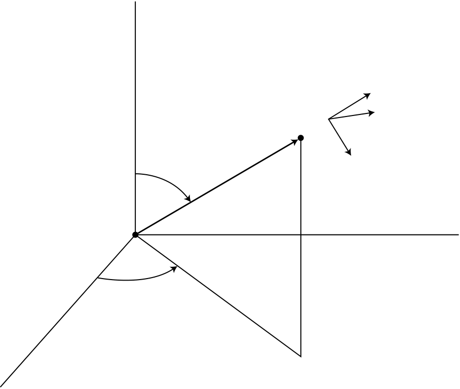
Suppose that the position of a particle P is specified by the values of its cylindrical coordi-nates (r, φ, z). We see from Fig. 1.1 that the position vector r is

r = rer + zez (1.15)

r	P	eφ
r	P	er

O		y

Figure 1.1.

5

v = ˙r = ˙rer + r˙φeφ + ˙zez (1.18)

Similarly, noting that

velocity and acceleration equations for plane motion using polar coordinates.

Spherical coordinates

r	P	eq

O	y

x

Figure 1.2.

˙er = ω × er =˙θeθ +˙φ sin θ eφ ˙eθ = ω × eθ = −˙θer +˙φ cos θ eφ ˙eφ = ω × eφ = −˙φ sin θ er −˙φ cos θ eθ	(1.23)

Then, upon differentiation of (1.21), we obtain the velocity

	(1.25)

Suppose a particle P moves along a given path in three-dimensional space. The position of the particle is specified by the single coordinate s, measured from some reference point along the path, as shown in Fig. 1.3. It is convenient to use the three unit vectors (et, en, eb) where et is tangent to the path at P, en is normal to the path and points in the direction of the center of curvature C, and the binormal unit vector is

eb = et × en	z	C	ρ	et		(1.26)
eb = et × en	z	C	en	P		(1.26)

O	y

Figure 1.3.

7	Particle motion

	(1.27)

	(1.28)

Thus, we find that the acceleration of the particle is

a = ˙v = ¨set + ˙s˙et = ¨set +˙s2 ρen (1.29)

(1.31)

Relative motion and rotating frames

where we note again that the frame A is moving in pure translation.

Now consider the general case in which the moving xyz frame (Fig. 1.4) is translating and rotating arbitrarily. We wish to find the velocity and acceleration of a particle P relative

		z

Z
r y

r
w

O	R	x

9	Particle motion

Thus, we obtain the important result:

a = ˙v =¨R + ˙ω × ρ + ω × (ω × ρ) + ( ¨ρ)r + 2ω × ( ˙ρ)r (1.42)

vB	B

rB	r	vA	A
C	rA	vA	A

	Introduction to particle dynamics

extension thereof, at which the velocity is momentarily zero. This is the instantaneous center of rotation.

Example 1.1 A wheel of radius r rolls in planar motion without slipping on a fixed convex surface of radius R (Fig. 1.6a). We wish to solve for the acceleration of the contact point on the wheel. The contact point C is the instantaneous center, and therefore, the velocity of the wheel’s center O′is

v = rωeφ (1.44)

O′		O

C	R	ω	O′		R
			O′
O			C
O			er
(a)			(b)

11

								(1.45)
so we find that
rω ˙φ = R + r								(1.46)
= r ˙ωeφ −r2ω2 R + rer (1.48) Similarly C, considered as a point on the rim of the wheel, has a circular motion about O′,
								(1.49)
Thus, the instantaneous center has a nonzero acceleration.								(1.50)
Now consider the rolling motion of a wheel of radius r on a concave surface of radius R (Fig. 1.6b). The center of the wheel has a velocity
								(1.51)
								(1.52)
								(1.53)
aO′ = (R − r) ¨φeφ − (R − r) ˙φ2er = r ˙ωeφ −r2ω2 R − rer aC/O′ = −r ˙ωeφ − rω2er Thus, we obtain
a	r	r2	�		�	Rr	�	(1.56)
C = −	� +	R − r	�	r = −	�	R − r	�	(1.56)

12	Introduction to particle dynamics

O′	f	r

k
C eq


r which rolls without slipping on a horizontal circular track of radius R (Fig. 1.7). The plane of the wheel remains vertical and the position angle of P relative to a vertical line through the center O′is φ. Let us choose the unit vectors er, eθ, k, as shown. They rotate about a vertical axis at an angular rate ω which is the rate at which the contact point C moves along the circular path. Since the center O′and C move along parallel paths with the same speed, we can write
		(1.57)

ω =r R	(1.58)

˙ω =r R

13

˙ω × ρ = −r2	¨φ sin φ er

and

2ω × ( ˙ρ)r = −2r2		(1.66)

(1.69)

where k is a constant (Fig. 1.8). Let us find an expression for its acceleration. Also solve for the radius of curvature of the spiral at a point specified by the angle θ.

et	er		en		r	y
et	eq	α	en		r	y

14	Introduction to particle dynamics

		(1.73)

		(1.74)
The radius of curvature at P can be found by first establishing the orthogonal unit vectors (et, en) and then finding the normal component of the acceleration. The angle α between the unit vectors et and eθ is obtained by noting that
tan α =vr vθ	=˙r r˙θ= k ˙θ kθ˙θ= 1	(1.75)

(1.77)

15	Systems of particles
	From (1.29), using tangential and normal components, we find that the normal accelera-tion is
			(1.80)

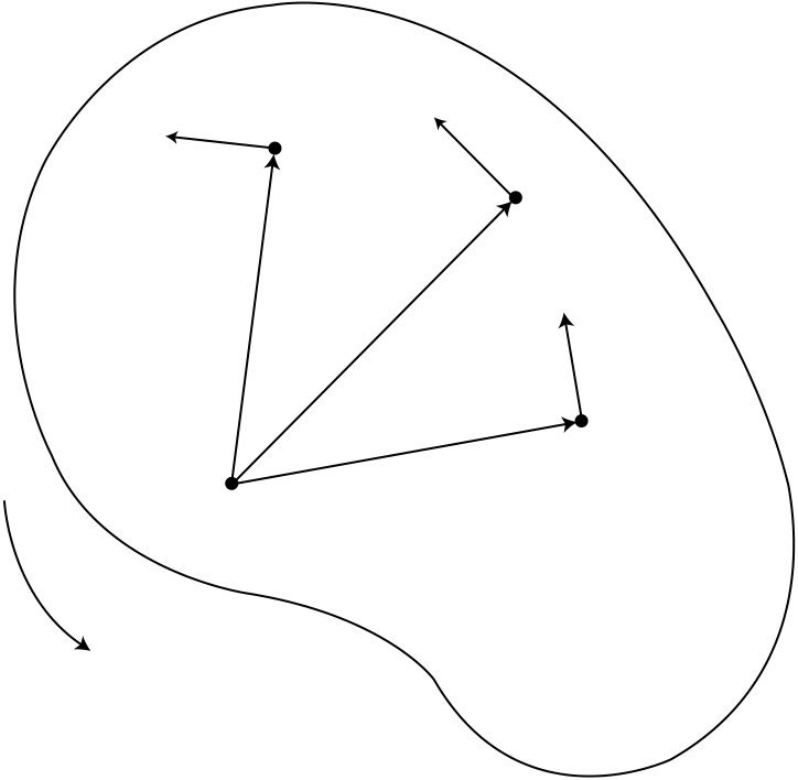
1.2

Systems of particles

Fi	mi

fij

O	ri	rc	rj		fji	mj
O	ri	rc	rj		fji

Figure 1.9.