
Logistic regression including kernel meth-ods
Machine Learning Theory (CS 6783)
Lecture 7 : Rademacher Complexity
| ES | �LD(ˆyerm) − inf f∈FLD(f)� | ≤2 nESEϵ | �f∈F sup | n � |
|---|
{z1, . . . , zn} as
ˆRS(G) := 1 nEϵ�sup
Proposition 1. For any sample S = {z1, . . . , zn} and any classes G , H mapping instances in Z
to reals :
1
Proof.
| �supg∈H | �n t=1ϵtg(zt)� | ≤1 nEϵ | �supg∈G | �n t=1ϵtg(zt)� |
|---|
g∈G�ϵt(g(zt) + h(zt))�
= 1 nEϵ�sup
3. cvx(G) = {z �→ Eg∼π [g(z)] : π ∈ ∆(G)}
ˆRS(cvx(G)) = 1 nEϵ�π∈∆(G)
= 1 nEϵ�sup
g∈G�ϵtg(zt)�
of the class of predictors. That is ˆRS(ℓ ◦ F) ≤ LˆRS(F)
2
|
||
|---|---|---|
Repeating the above argument we remove φ1, . . . , φn−1 and so, we conclude that
|
||
| 3 | ˆRS(F) = 1 nEϵ�f:∥f∥1≤R
|
|---|
{e1, −e1, e2, −e2, . . . , ed, −ed}. Hence by Proposition 1 (4) we have that
Example applications : Lasso, SVM, ridge regression, Logistic Regression (including kernel meth-
have,
ES�LD(ˆyerm) − inf f∈FLD(f)�≤ 2L ESEϵ�f∈F sup�ϵtf(xt)� n
subject to ∥f∥2 ≤ R
This corresponds to class F given by linear predictors with Hilbert norm constrained by R
Corresponds to linear predictor with ℓ1 norm constrained by 1
4
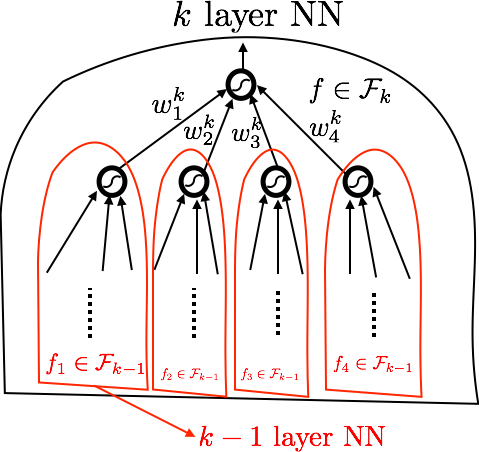
ˆRS(Fi) = 1 nEϵ ∀j, fj∈Fi−1 ∥wi∥1≤Bi sup � n
�ϵtwi jσ(fj(xt))
≤2Bi
nEϵ
nEϵ
f∈Fi−1
supsup
sup
ϵtσ(fj(xt))
j ������ϵtσ(fj(xt))������� ������
5


