

Levis factor measuring wireless link burstiness
@scale: Insights from a Large, Long-Lived Appliance
Energy WSN
Abstract
We present insights obtained from conducting a year-long, 455 meter deployment of wireless plug-load electric meters in a large commercial building. We develop a stratified sam-pling methodology for surveying the energy use of Miscella-neous Electric Loads (MELs) in commercial buildings, and apply it to our study building. Over the deployment period, we collected over nine hundred million individual readings. Among our findings, we document the need for a dynamic, scalable IPv6 routing protocol which supports point-to-point routing and multiple points of egress. Although the meters are static physically, we find that the set of links they use is dynamic; not using such a dynamic set results in paths that are twice as long. Finally, we conduct a detailed sur-vey of the accuracy possible with inexpensive AC metering hardware. Based on a 21-point automated calibration of a population of 500 devices, we find that it is possible to produce nearly utility-grade metering data.
with the expectation that they will work to produce use-ful, scientifically-relevant data. Deploying these systems at scale requires rigorous attention to both engineering and de-ployment management. Recent studies have begun to show successes and failures [4, 11, 17] as well as offering practical guidance on deployments, continuing the sequence of papers performing science in the real world [31, 35].
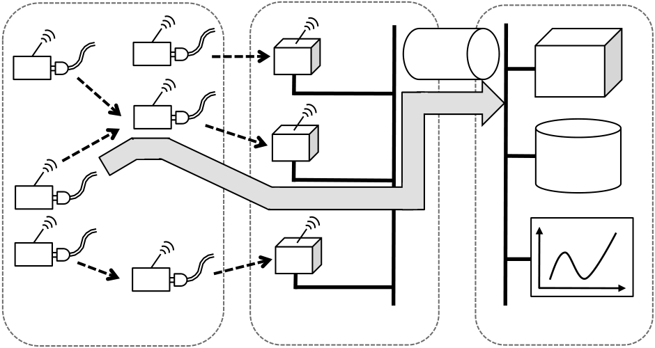
In this paper, we present results and insights from a mas-sive application, developed and deployed over the past two years. This application consists of 455 wireless energy plug-load meters and 7 load-balancing routers deployed across four floors of a commercial building for the past year. It was motivated by a need for a better understanding of the power consumption and usage patterns of electric plug-loads, or “miscellaneous electric loads.” These are estimated to make up nearly 30% of the electric load in commercial build-ings [32], but are difficult to study because they are so nu-merous and diverse. They are a good target for a wireless sensor network because they require both high density and a large number of metering elements.
| Keywords |
|---|
1. INTRODUCTION
More than a decade after wireless sensor networks emerged as a topic of
research, much progress has been made in un-derstanding the contours of
the field. There is now a large body of work from which to draw
inspiration and ideas. From the early “let chaos reign” days to the
current state-of-the-art, the field has evolved to the point where it is
pos-sible to deploy large-scale applications over a long period
Permission to make digital or hard copies of all or part of this work for personal or classroom use is granted without fee provided that copies are not made or distributed for profit or commercial advantage and that copies bear this notice and the full citation on the first page. To copy otherwise, to republish, to post on servers or to redistribute to lists, requires prior specific permission and/or a fee.
goals of the deployment require consideration of the accu-racy required by the meters; we developed an extensive automated calibration procedure that could be efficiently applied to hundreds of meters to achieve better than 2%
For example, an “LCD computer display” is a product type in the “Display” category, which is part of the end use “Elec-tronics.” The inventory categorized every plug-load in the building according to this taxonomy, resulting in the identi-
| accuracy. | |||
|---|---|---|---|
| 2.2 | |||
|
|||
In the remainder of the paper we first present an overview of the science goals and methodology of our study. We then present our system design, noting where we have learned from mistakes published in the past and pointing out how simplicity is key to conducting large deployments with lim-ited resources. In the body of the paper, we examine the lessons learned by deploying our large system, and how being driven by energy science (in addition to computer science) goals led to new insights.
• Study usage correlations between devices, e.g., com-puter, display, and lighting within the same occupant’s
| “miscellaneous” category (MELs). |
|
|---|
We developed a multi-stage, stratified random sampling approach to select devices for metering. Devices were first divided into stages by physical location or organization own-ing the devices. For each stage, a subset of devices were then selected from a stratified sample by Device Category to meet our data collection objectives. A stratified sample is critical because a simple random sample would result in metering a large number of uninteresting devices (e.g., computer speak-ers, external disk drives) instead of devices with significant energy use such as computers or LCD displays.
In the second phase of the study, we deployed a total of 455 meters on the selected devices. The deployment took ap-proximately 120 person-hours. No effort was made to deploy meters to ensure network connectivity, but load-balancing routers (LBRs) were placed with connectivity and hop count in mind. Once the meters were in place, we had only lim-ited opportunities to perform on-site troubleshooting. This made our remote debugging setup more important.
| 3. | |||
|---|---|---|---|
| truth when comparing various sampling approaches. |
|
||
to the diversity of devices, a standardized system of iden-tifying and recording MELs is essential for inventory and energy data analysis. We updated an extensive taxonomy developed in [23] to include new device types found today, such as tablet computers. The taxonomy consists of three

|
|||||||||||||||||||||||||||||||||||||||||||||||||||||||||||||||||||||||||||||||||||||||||||||||||||||||||||||||||||||||||||||||||||||||||||||||||||||||
|---|---|---|---|---|---|---|---|---|---|---|---|---|---|---|---|---|---|---|---|---|---|---|---|---|---|---|---|---|---|---|---|---|---|---|---|---|---|---|---|---|---|---|---|---|---|---|---|---|---|---|---|---|---|---|---|---|---|---|---|---|---|---|---|---|---|---|---|---|---|---|---|---|---|---|---|---|---|---|---|---|---|---|---|---|---|---|---|---|---|---|---|---|---|---|---|---|---|---|---|---|---|---|---|---|---|---|---|---|---|---|---|---|---|---|---|---|---|---|---|---|---|---|---|---|---|---|---|---|---|---|---|---|---|---|---|---|---|---|---|---|---|---|---|---|---|---|---|---|---|---|---|
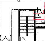
Figure 1: The third floor of the deployment. Small boxes are meters, while the two stars are LBRs.
msp430 microcontroller integrated with an 802.15.4 radio backhaul capacity by deploying new meters and routers at and Analog Devices ADE7753 energy metering chip. Each will.
| 8W� | 0W� | LBR | IPv6 | VPN | |||
|---|---|---|---|---|---|---|---|
| 3W� | |||||||
| 4W� | LBR |
|
|
||||
| 3.1 | |||||||
| UDP data path | |||||||
| 9W� | |||||||
| 0W� | LBR | ||||||
| Back haul tier | |||||||
|
|
||||||
ternet where they reach the database, located in a the-air image update utility, in practice it was rarely used
datacenter. since we could update parameters without reflashing the
| out any extra configuration. This is a key result of our use | 3.2 | ||
|---|---|---|---|
| of the IP architecture. |
|
||
vices make up a single IPv6 subnet where all devices partic-ipate in the routing protocol called HYDRO [8], designed to provide efficient any-to-any IPv6 routing over constrained
One of the most important aspects of sensing is the no-tion of time. It allows correlation of readings across meters. Even though approaches to time synchronization of vari-ous sophistication have been used successfully [4, 19, 25], problems with it are well documented [35]. Given our re-quirements, our approach was very simple. Therefore, we
included redundant clocks and counters to distinguish the various events we expected in such a large deployment; these counters are presented in Table 1.
|
|
|---|
4. NETWORKING INSIGHTS
An important component of our network is the routing protocol that provisions routes from the individual meters towards the edge of the access network. The protocol needed to be reliable and perform at a scale of hundreds of individ-ual meters. We used HYDRO [8], a conceptual predeces-sor to the RPL protocol currently being advanced in the IETF [36]. HYDRO builds a directed acyclic graph (DAG) towards a set of load-balancing routers (LBRs). Traffic orig-inating from inside the network is routed down this DAG to one of the LBRs, where further routing decisions are made. Traffic originating from an LBR or another network is first routed to the “nearest” LBR, and then source-routed to its final destination.HYDRO contains numerous mechanisms to improve reli-ability and scalability in the face of shifting link conditions and deployment sizes. Each router maintains a list of po-tential next-hop default routes and will attempt delivery to several of them, using link-layer acknowledgements to de-termine whether a particular packet was delivered. Each embedded router also maintains only a subset of its neigh-bor set to limit the amount of state and periodically attaches this information to outgoing data packets. The LBRs use this information to build a view of the link state of the net-work and construct source routes back into the network.
|
||||
|---|---|---|---|---|
|
||||
| deployments. | ||||
|
||||
Our key insight was the value of configuration, not repro-gramming. In the two or so years since our mote software was “released to manufacturing,” we have not developed a new image; instead we have been able to work around the
|
|---|
ware. Because of the ability to change parameters, we have been able to deploy meters in other systems not discussed here with differing needs but the same software. This results
| in a significantly smaller testing surface. |
|---|
Finally, IPv6 allowed us to develop compact implementa-tions of many services wished for in previous deployments, like a configuration manager and a software updater. Al-though some of these were less efficient than the state-of-the-art, they worked when required at a very large scale.
sages as would be required in an on-demand protocol. This is somewhat in opposition to the networking structure that has emerged in recent years in TinyOS, positing that collec-tion (MP2P) and dissemination (P2MP) are the dominant traffic patterns. Although these are invaluable and common traffic patterns, at times it is simply convenient to contact a single node individually.
| to be offline for various reasons. | Data delivery rate | 1 | ||||||||
|---|---|---|---|---|---|---|---|---|---|---|
|
|---|
|
|
|---|---|
| Building shutdowns | |
|
|
|
|
| 6 | Mean router degree | 03/26 | 04/02 | Proportion of motes | 1 | 2 | 3 | 4 | 5 | 6 | 7 | midnight |
|
||||
|---|---|---|---|---|---|---|---|---|---|---|---|---|---|---|---|---|---|
|
|||||||||||||||||
| 5.5 | |||||||||||||||||
| 5 | |||||||||||||||||
| 4.5 | |||||||||||||||||
| 4 |
|
||||||||||||||||
|
|||||||||||||||||
| 3.5 | |||||||||||||||||
| 3 | Mean network shortest path | 8 | |||||||||||||||
| 03/05 | 03/12 | 03/19 | |||||||||||||||
| Date | Routing depth (ETX) | ||||||||||||||||
| number of links |
|
|
03/31 | 04/03 | number of links explored | 1000 500 |
|||||||||||||||||||||||||||||||||||||||||||||||||||||||||||||||||||||||
|---|---|---|---|---|---|---|---|---|---|---|---|---|---|---|---|---|---|---|---|---|---|---|---|---|---|---|---|---|---|---|---|---|---|---|---|---|---|---|---|---|---|---|---|---|---|---|---|---|---|---|---|---|---|---|---|---|---|---|---|---|---|---|---|---|---|---|---|---|---|---|---|---|---|---|---|---|---|
to-end acknowledgements are not a panacea for data reli-ablity problems unless much care is taken managing send buffers on the mote to guarantee all data is delivered in the face of connection resets and timeouts. Transport- and application-layer protocol designs currently in development (for instance, CoAP [26]) should be evaluated to ensure that they provide appropriate mechanisms for caching between
| 4.3.2 |
|
network segments, especially if they are designed to work |
|---|---|---|
| over UDP. It is an open question of how to merge the buffer- |
The final question was whether the effort to discover and track these variable links was “worth it.” That is, does the set of churn links improve routes to the LBRs? The answer is a resounding“yes.” If we were to consider only the links in the static set, i.e., those continuing to appear after a week, the network diameter increases by a factor of 2.1: from an ETX of 4.6 to 9.9.
ing and end-to-end demands of TCP with the constrained resources of embedded systems.
We used these goals to guide the design and development of an automated calibration process. It uses eight different resistive loads from 2W to 100W, actuated by a computer-controlled relay to create 21 calibration points between 0W
| 4.4 |
|
|
|---|---|---|
| The process of developing a calibration function revealed a couple of key insights. First after analyzing raw data from |
|
|---|
| ear behavior but only over limited domains. In fact, a single | CDF of Meters (%) | 0.5 | 1 | 1.5 | 7.0 Watts | 3 | ||
|---|---|---|---|---|---|---|---|---|
| linear function over the entire range of loads cannot meet our | ||||||||
| accuracy target. Therefore, single-point calibration is insuf- |
|
|||||||
| ficient. Instead, a piecewise linear function using multi-point | ||||||||
| calibration as shown in Figure 6 may be used, consisting of |
|
|||||||
| three portions, where the first only ensures that the meter | ||||||||
| returns a zero reading at zero load, and the boundary be- | ||||||||
| tween the second and third segment is chosen to minimize | ||||||||
| the overall error in the calibration. Although more segments | ||||||||
| in the function would decrease error, there is risk of over- | ||||||||
| fitting as well as unnecessary complexity. The calibration | 50.8 Watts | |||||||
| coefficients are stored on each meter so that future readings | 75.8 Watts | |||||||
|
216.5 Watts | |||||||
| are provided in engineering units (mW) for easier analysis. | ||||||||
|
2.5 | |||||||
| Calibration Error (W) |
| examined across all meters. The error of this calibration pro- | ||
|---|---|---|
| cedure for the entire population of 455 meters is shown in | ||
| Figure 7. The plot shows cumulative distribution functions |
at four load levels. At low loads, we achieve absolute errors
of less than 1W for virtually all of the meters calibrated. Additionally, more than 75% of meters are within 2% of the
| I44H |
|
|
||||||
|---|---|---|---|---|---|---|---|---|
| 2/.$"'"/' | ||||||||
| *+=+&+$1+'*+#:'?/@+&'AHF | ||||||||
|
||||||||
|
||||||||
| !+,5+$"'+$%2/.$"-' | ||||||||
| -+:+1"+%'=/&' | ||||||||
| 1/$".$<."> | ||||||||
| GH | ||||||||
| *+#:'?/@+&'AB&C."&#&>'BD5+'E$."-F | ||||||||
| Figure 6: | &"!! | |||||||
puters, uses about 60% of its energy outside working hours the manifold use of statistics” to have frequent state reports
at this facility. Considering that only 10% of the computers available for potential debugging efforts [17]. In our study,
| Computers |
|
|
|
|---|---|---|---|
| Other |
|
||
| 50% of energy |
|
||
| Displays | ||
|---|---|---|
| 12% of energy | ||
|
|
| energy-efficient products are used in a building. |
|
|---|
equipment, price and efficiency are not tightly correlated. Consider computer displays. A comparison of the on-mode
of link dynamics. Zhao and Govindan characterize the size and behavior of “grey zones” of intermittent performance in low-power links, while Son, et al. extend this understanding to multiple contending senders [27, 37]. Srinivasan, et al.
decrease by 40%. synthesize these results into a more detailed understanding
There are also several takeaways which should inform fu-ture protocol design. It is still somewhat unusual to connect large subnetworks of devices directly to the broader Inter-net but gave us host of advantages in terms of debugging and visibility; this may cause researchers in the embedded space to examine transport protocols which can provide bet-ter end-to-end guarantees than either UDP or TCP while continuing to impose a very low burden on the low-power and lossy network segments. Incorporating reliability at ev-ery layer of design is common practice in other domains; we expect it to become common here as well.
The result of this work is to allow deployments at larger scales. We have presented results from @scale; one of the largest deployment in terms of mote-years yet published. We were successful in achieving our science goals while testing several hypotheses about network dynamics, and reinforced emerging design practice on the construction of this type of
[10] Electronic Product Design, Inc. Plm-1 power meter.
.
| network. |
|
|---|
Acknowledgements
[4] G. Barrenetxea, F. Ingelrest, G. Schaefer, and M. Vetterli. The hitchhiker’s guide to successful wireless sensor network
deployments. In Proceedings of the 6th ACM conference on Embedded network sensor systems, pages 43–56, New York, NY, USA, 2008. ACM.[5] J.-C. Bolot. End-to-end packet delay and loss behavior in the internet. SIGCOMM Comput. Commun. Rev., 23:289–298, October 1993.
[19] M. Mar´oti, B. Kusy, G. Simon, and ´Akos L´edeczi. The flooding time synchronization protocol. In SenSys ’04: Proceedings of the 2nd international conference on Embedded networked sensor systems, New York, NY, USA, 2004. ACM Press.
[20] J. Martocci, P. D. Mil, N. Riou, and W. Vermeylen. RFC 5867: Building automation routing requirements in low-power and lossy networks, 2010.
.
[24] J. Ortiz and D. Culler. Multichannel reliability assessment in real world wsns. In Proceedings of the 9th ACM/IEEE International Conference on Information Processing in Sensor Networks, New York, NY, USA, 2010. ACM.
[26] Z. Shelby, K. Hartke, C. Bormann, and B. Frank. Constrained
Application Protocol (CoAP). Internet-Draft
draft-ietf-core-coap-07, Internet Engineering Task Force, July 2011.
Work in progress.
[27] D. Son, B. Krishnamachari, and J. Heidemann. Experimental Analysis of Concurrent Packet Transmissions in Low-Power Wireless Networks. Tech Report ISI-TR609, Viterbi School of Engineering, University of Southern California, 2005.
[31] G. Tolle, J. Polastre, R. Szewczyk, D. Culler, N. Turner, K. Tu, S. Burgess, T. Dawson, P. Buonadonna, D. Gay, and W. Hong. A macroscope in the redwoods. ACM Sensys, 2005.
[33] A. Wang, C. Huang, J. Li, and K. W. Ross. Queen: Estimating packet loss rate between arbitrary internet hosts. In 10th International Conference on Passive and Active Network Measurement, volume 5448 of Lecture Notes in Computer Science. Springer, 2009.


