June phased array antenna patternspart grating lobes and beam squintpeter delos

Vol 54 No 2, June 2020

	0	Grating Lobes with the d = 0.7 case λ			d
	–5	Grating Lobes with the d = 0.7 case λ			λ 0.5
	–10	–40	–20	0
	–10
	–15
squint. Grating lobes can be hard to visualize, so we’ll draw on their similarity	–15
with signal aliasing in digital converters, then use that to think of a grating lobe	–20
	–20
	–25

					80
	–30
	–30
	–35
typical systems.	–35
An Introduction to Grating Lobes	–40
	–40	Angle (°)

Analogy to Sampled Systems

An analogy to visualize grating lobes is to think of aliasing in a sampled system. In an analog-to-digital converter (ADC), undersampling is often used when frequency planning a receiver architecture. Undersampling involves purposefully reducing the sample rate (fS) such that the sampling process translates frequencies above fS/2 (the higher Nyquist zones) to appear as aliases in the first Nyquist zone. This causes those higher frequencies to appear as if they were at a lower frequency at the output of the ADC.

∆Φ = 2�dsinθ λ			(1)
∆Φ = 2�dsinθ λ				θ = arcsin	m×	(5)
				θ = arcsin	m×	(5)
	∆Φ	× λ d	(2)
	2�	× λ d	(2)

every 2π. So, we could replace ∆Φ with (m × 2π + ∆Φ) in the beam steering

θ = arcsin	m× 2� + ∆Φ
	m× 2� + ∆Φ	exist. For example, if λ/d = 0.66 (that is, d = 1.5λ), then real arcsin solutions
	2�
	2�	would exist for m = 0 and for m = ±1. That m = ±1 is the second solution, which is

m× 2� + ∆Φ	λ		()
2�	×d		()

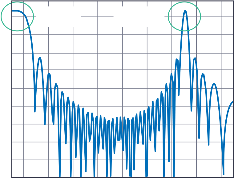
If we do so, then all the spatial images (that is, m = ±1, ±2, etc.) will produce non-real arcsin results, and we can ignore them. But if we can’t do this, and therefore some values of m > 0 produce real arcsin results, then we end up with multiple solutions: grating lobes.

Not Real	2π	y

–2	–1		o 0	x	1	y = arcsin (x)
–2	–1		o 0	x	1	2

0
–5
–10
–15
–20
–25
–30
–35
–40
–40	–80	–60	–40	–20	0	20	40	60	80

Angle (°)

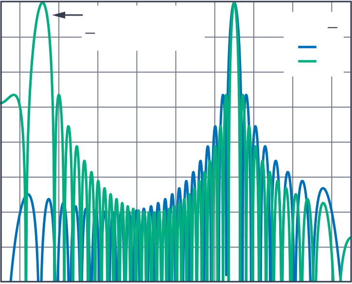
θ = arcsin m , for ∆Ф = 0 λ
d

So for Example: λ/d = 0.66
0 = Actual Lobe
X = Grating Lobes

2

First, recall how the phase changed with steering angle in Figure 4 from Part 1.				15		This is the		This is the
We saw ∆Φ range from 0 to ±π as the main lobe deviated from mechanical						This is the		This is the
						Grating Lobe		Desired Lobe
boresight. Therefore,				10
	(6)			10
				5
2�			Directivity (dBi)	0	–80	–60	–40	–20	0	20	60
will range				0
from 0 to ±0.5 ×	for m = 0	(7)		–5
from 0 to ±0.5 ×	for m = 0	(7)		–10
And for \|m\| ≥ 1, it will always be something beyond				–15
	(8)			–20
This restricts the minimum permissible λ/d if we want to keep the entire arcsin				–25
argument > 1 for all \|m\| ≥ 1. Consider two cases:
X If λ/d ≥ 2 (that is, d ≤ λ/2), then you could never have multiple solutions,

It is an interesting trade-off that will be explored in the next section.

Element Spacing Considerations

m× 2� + ∆Φ	λ		(9)
2�	×d

±1 × 2� +	2�dmaxsinθmax
	λ	×	λ	= 1	(10)
	2�		dmax

	(11)
Then solving for dmax λ

			(12)
	1 + \|sinθmax\|		(12)

This dmax is the condition for no grating lobes in the reduced scan angle (θmax), where θmax is less than π/2 (90°). For example, if the signal frequency is 10 GHz and we need to steer ±50° without grating lobes, then the maximum element spacing is:

dmax =		(13)

There are also antenna architectures worth noting that attempt to overcome the grating lobe problem by producing a nonuniform element spacing. These are categorized as aperiodic arrays, with spiral arrays as an example. For mechanical antenna construction reasons, it may be desirable to have a com-mon building block that can be scaled to a larger array, but this would produce a uniform array that is subject to the grating lobe conditions described.

Beam Squint

VISIT ANALOG.COM	3

0	40	9 GHz	0	40	9 GHz
–5		9 GHz	–5		9 GHz
		10 GHz			10 GHz
		11 GHz			11 GHz
		80	–10		80
–15			–15


–30			–30


0			0
	Angle (°)			Angle (°)
	(a) θ = 20			(b) θ = 40

–5

Amplitude (dB)

–30

–35

–40	10	20	30	40	50	60	70	80
0	10	20	30	40	50	60	70	80

					20	f	0.8
and therefore no means to produce any beam squint. Therefore, the amount of					15		0.8
							0.9
beam squint must be a function of angle, θ, as well as the frequency variation.						f0	1.1
							1.2
					10		1.2
					5		10
					5
					0
					0
					–5
beam direction deviation, beam squint, can be calculated as
∆θ = arcsin	f0	sinθ0	– θ0	(14)
	f0				–10
	f				–10
	f				–15


					–20
					–20
					0

Figure 6. Beam squint vs. beam angle for several frequency deviations.

4	Phased Array Antenna Patterns—Part 2: Grating Lobes and Beam Squint

Beam Squint Considerations

The beam squint, deviation in steering angle vs. frequency, is caused by approxi-mating a time delay with a phase shift. Implementing beam steering with true time delay units does not have this problem.

	shifter quantization errors.

shifter over a time delay unit? Typically, this comes down to design simplicity and IC availability of phase shifters vs. time delays. Time delays are implemented in some form of transmission line and the total delay needed is a function of the aperture size. To date, most available analog beamforming ICs are phase shift based, but there are families of true time delay ICs emerging and these may become much more common for phased array implementations.

digital beamforming algorithms. Therefore, a phased array architecture where Artech House, 2005.

every element is digitized would lend itself naturally to overcome the beam squint problem, while also providing the most programmable flexibility. However, the power, size, and cost of such a solution can be problematic.

Bob Broughton started at Analog Devices in 1993 and has held positions as a product engineer and an IC design engineer, and is

currently the director of engineering in the Aerospace and Defense Business Unit. Prior to ADI, Bob worked at Raytheon as an RF

design engineer and at Peregrine Semiconductor as an RFIC designer. Bob graduated with a B.S.E.E. from West Virginia University

in 1984. He can be reached at bob.broughton@analog.com.

About the Author

Jon Kraft is a senior staff FAE in Colorado and has been with ADI for 13 years. His focus is software-defined radio and aerospace

phased array radar. He received his B.S.E.E. from Rose-Hulman and his M.S.E.E. from Arizona State University. He has nine patents

For regional headquarters, sales, and distributors or

	Ask our ADI technology experts tough questions, browse FAQs, or join a conversatioeerZone Online Support Community. Visit .