Hessian matrix independent ofh the parameters

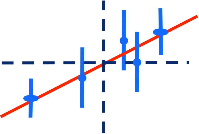
Review: Fit a line to N data points

€
	y = a (x − ˆ x ) + b								Pivot point:
									ˆx ≡	∑
										∑


	ˆ b	∑	yi σ i		2	,	Var ˆ b [ ]=
€	=		1 σ i	2			Var ˆ b [ ]=	∑	1 σ i

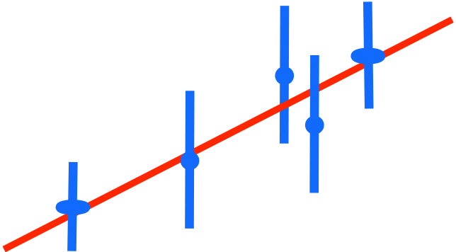
For slope a, set b=0 and find a by optimal scaling:

	ˆ a =	∑	yi xi − ˆ x ) σi			2			∑	1	2 σ i
		∑	(xi −ˆ x )	2 σ i	2					(xi −ˆ x )
		∑	(xi −ˆ x )	2 σ i	2					(xi −ˆ x )

	α 0 = ˆ	∑	(		yi − ˆ α 1 P1(xi) )P0(xi) σi				2					1		ˆ x
					yi − ˆ α 1 P1(xi) )P0(xi) σi									P0			Pivot point:
€					∑	P0	2(xi) σ i	2					∑	P0	2(xi) σ i	2
	α 1 = ˆ	∑	(	yi − ˆ α 0 P0(xi) )P1(xi) σi					2	,		∑
	α 1 = ˆ	∑	(	∑		P1 2(xi) σ i		2	2	,		∑

	LINEAR REGRESSION:										y	=
	LINEAR REGRESSION:													∑αk Pk(x)
														∑αk Pk(x)

χ2≡		N	#	yi −(a xi + b)							&
		∑	#								&
			% $								( '

				σ i
		i=1		σ i
							∑	x y − a x − b (										y = a x + b
0 = ∂ χ 2∂ b= −2							∑	(y − a x − b					)σ 2					y = a x + b
0 = ∂ χ 2∂ b= −2							∑	(y − a x − b					)σ 2					€	b	χ2(a,b)

a	∑x2 σ 2					+ b∑x σ 2						=	∑		x y σ2
a	∑x σ 2				+ b∑1 σ 2							=						€	ˆb
Matrix form:																		€	ˆb
#								Σx /σ2				&	#	a				Σx y /σ2
%												(	#				%
%												(	%				%
% $								Σ 1/σ2					%	b				Σ y /σ2	ˆa
% $								Σ 1/σ2					$	b		'		Σ y /σ2	ˆa
H α									=		c(y)
H α									=		c(y)							( c = correlation vector )
										=	H							( c = correlation vector )

The Hessian Matrix

H jk ≡1 2				χ2≡	N
					∑
					∑			 
					i=1
	∂aj∂ak				i=1
	∂aj∂ak

							(y − a x − b ) σ 2
∂2χ2 ∂ a2 = 2 i∑							(y − a x − b ) σ 2
∂2χ2 ∂ a2 = 2 i∑				i∑		    
∂2χ2 2			xi€ 2 /σ i 2	i∑
∂2χ2 2		   i∑

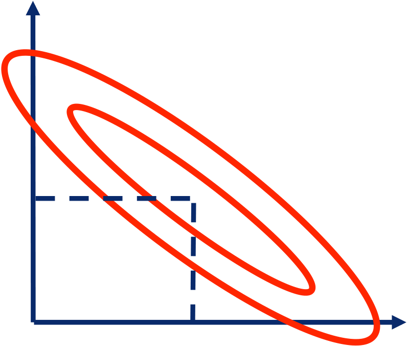
Parameter Uncertainties Hessian matrix describes the curvature of the χ2 surface :

χ2(α) = χ2( ˆ α ) +	j,k∑	( α j − ˆ α j	)Hj kαk− ˆ α k		1	∂2χ2
						∂aj∂ak

	the parameters, and χ2 surface is parabolic. For a one-parameter fit:
€
€	if ˆ α minimizes χ 2, then Var( ˆ α ) =

Cov(aj,ak) = H−1 "#

General Linear Regression 

Scale M Patterns	M
	∑

Example:	Polynomial: y(x) = a0 + a1 x + a2 x2+ ...+ aM −1 xM −1
Example:	N		=	N	σ i 2yi−  	M
χ2≡	∑			∑		∑

		 
	i=1	 		i=1		j

Normal Equations:

				2	N	#		M	aP(x)			Pk(xi)
					∑	#		∑
						%		∑			(
				= −		% $		∑
				= −	i	% $		j
M	#	N	Pji Pki					N	yi Pki	Pki ≡ Pk(xi)
∑	#	∑						∑
	%	∑
	% $						=								N
j		i						i
j		i						i	H jk =			N	Pji Pki	c(y)
M												N
∑			H jk aj = ck(y)									∑			∑
∑			H jk aj = ck(y)									∑	2 σ i	k =	∑
j												i	2 σ i	k =	i


Linear Model :y(x) =				M∑αk Pk (x)
k
H1	∂2χ2		N
	∂α j ∂αk	=	∑
	∂α j ∂αk	=	i=1

Elliptical χ2 contours, unique solution by linear regression (matrix inversion).

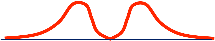
Non - Linear Models :

		j,k∑	(αj− ˆαj	)Hj kαk− ˆαk	)
H1	∂2χ2	depends on the non-linear parameters.
	∂α j ∂αk	depends on the non-linear parameters.

				A and B are scale parameters.
				∂µ ∂ A= g
				∂µ ∂ A= g
	∂µ	+ Δσ ∂µ ∂σ		x0 and σ are non-linear parameters.
		+ Δσ ∂µ ∂σ
∂ A= g∂µ			€
∂ A= g∂µ			€
∂ B=1 ∂µ∂σ = A g η2 /σ
				∂µ
				∂σ

Simplex = cluster of M+1 points in the	3	2	6	8
	3
	1
	1

place with lower χ2 .	4	5	7
3. Repeat until converged.	4	5	7

3. Take a random step, e.g. using a Gaussian

random number with same σi (and
covariances) as “recent” points.

MCMC requires no derivativesJ Easy to code J

MCMC generates a “chain” of points tending to move downhill, then settling into

0.5
0

-1
-1	0.6	0.8	1	1.2

	-0.02 0 0.02 0.04 0.06 0.08

0.1
0.12
0.14

0.95	1