
Box plot command ggplot geom package basic ggplot
BIOSTATS'640'–'Spring'2018'''''''''''''''''''''''''''''''''''''''''''''''''''''''''''''''''''''''''''''''''''''Introduction'to'R'–'Data'Description'
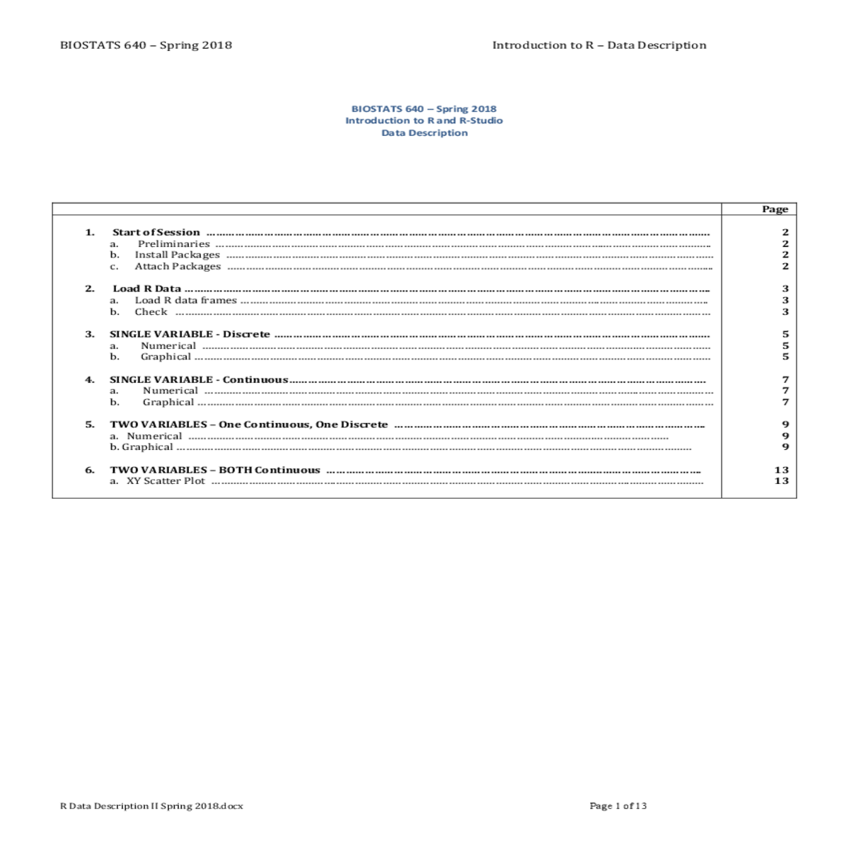
BIOSTATS'640'–'Spring'2018'
Introduction'to'R'and'R-Studio'
Data'Description'
| Page! | ||||||||
|---|---|---|---|---|---|---|---|---|
|
2! 2! ! 5! 7! 7! !
|
|||||||
'
|
|---|
library(DescTools)
library(psych)'
|
|---|
| 2. Load R Data! |
|---|
# 2b. Check
# str(DATAFRAME) to check structure of dataframe'
str(ivf)'
# tail(DATAFRAME) to display last 6 rows'
tail(ivf)'
|
|---|
R'Data'Description'II'Spring'2018.docx''''''''''''''''''''''''''''''''''''''''''''''''''''''''''''''''''''''''''''''''''''''''''''''''''''''''''''''''''''''''''''''''''''''''''''''Page 4 of 13'
BIOSTATS'640'–'Spring'2018'''''''''''''''''''''''''''''''''''''''''''''''''''''''''''''''''''''''''''''''''''''Introduction'to'R'–'Data'Description'
| 3.SINGLE VARIABLE - DISCRETE |
|---|
## level freq perc cumfreq cumperc'
## 1 male 326 50.9% 326 50.9%'
BIOSTATS'640'–'Spring'2018'''''''''''''''''''''''''''''''''''''''''''''''''''''''''''''''''''''''''''''''''''''Introduction'to'R'–'Data'Description'
|
|---|
'
R'Data'Description'II'Spring'2018.docx''''''''''''''''''''''''''''''''''''''''''''''''''''''''''''''''''''''''''''''''''''''''''''''''''''''''''''''''''''''''''''''''''''''''''''''Page 6 of 13'
|
|---|
|
|---|
|
|---|
'
|
|---|
|
|---|
BIOSTATS'640'–'Spring'2018'''''''''''''''''''''''''''''''''''''''''''''''''''''''''''''''''''''''''''''''''''''Introduction'to'R'–'Data'Description'
|
|---|
!
|
|---|
R'Data'Description'II'Spring'2018.docx''''''''''''''''''''''''''''''''''''''''''''''''''''''''''''''''''''''''''''''''''''''''''''''''''''''''''''''''''''''''''''''''''''''''''''''Page 10 of 13'
BIOSTATS'640'–'Spring'2018'''''''''''''''''''''''''''''''''''''''''''''''''''''''''''''''''''''''''''''''''''''Introduction'to'R'–'Data'Description'
'
R'Data'Description'II'Spring'2018.docx''''''''''''''''''''''''''''''''''''''''''''''''''''''''''''''''''''''''''''''''''''''''''''''''''''''''''''''''''''''''''''''''''''''''''''''Page 11 of 13'
'
|
|---|
BIOSTATS'640'–'Spring'2018'''''''''''''''''''''''''''''''''''''''''''''''''''''''''''''''''''''''''''''''''''''Introduction'to'R'–'Data'Description'
p32 <-p31 +theme_bw()
|
|---|


