
And calculated from the free space path loss formula
IEEE TRANSACTIONS ON SIGNAL PROCESSING 1
Relative Location Estimation in Wireless
Abstract
Self-configuration in wireless sensor networks is a general class of estimation problems which we study via the Cram´er-Rao bound (CRB). Specifically, we consider sensor location estimation when sensors measure received signal strength (RSS) or time-of-arrival (TOA) between them-selves and neighboring sensors. A small fraction of sensors in the network have known location while the remaining locations must be estimated. We derive CRBs and maximum-likelihood estimators (MLEs) under Gaussian and log-normal models for the TOA and RSS measurements, respectively. An extensive TOA and RSS measurement campaign in an indoor office area il-lustrates MLE performance. Finally, relative location estimation algorithms are implemented in a wireless sensor network testbed and deployed in indoor and outdoor environments. The measurements and testbed experiments demonstrate 1 m RMS location errors using TOA, and 1 m to 2 m RMS location errors using RSS.
IEEE TRANSACTIONS ON SIGNAL PROCESSING 3
To design a relative location system that meets the needs of these applications, several capa-bilities are necessary. The system requires a network of devices capable of peer-to-peer range measurement, an ad-hoc networking protocol, and a distributed or centralized location estima-tion algorithm. For range measurement, using received signal strength (RSS) is attractive from the point of view of device complexity and cost, but is traditionally seen as a coarse measure of range. Time-of-arrival (TOA) range measurement can be implemented using inquiry-response protocols [9][7]. In this article we will show that both RSS and TOA measurements can lead to accurate location estimates in dense sensor networks.
IEEE TRANSACTIONS ON SIGNAL PROCESSING 4
II. Network Estimation Bounds
F= −E∇(∇l(X|γ))T= fn,1 f1,1 ... · · ·
· · ·
... f1,n ...
| IEEE TRANSACTIONS ON SIGNAL PROCESSING | 5 |
|---|---|
| can be further reduced: when k ̸= l, there is at most one summand in (1) which is a function of | |
where IH(k)(l) is an indicator function, 1 if l ∈H(k) or 0 otherwise.
∂θ2 ∂2 |
(3) |
A. Conditions for a decreasing CRB
Intuitively, as more devices are used for location estimation, the accuracy increases for all of the devices in the network. For an n device network, there are O(n) parameters, but O(n2) variables {Xi,j} used for their estimation. The analysis of this section gives sufficient conditions to ensure the CRB decreases as devices are added to the network. Consider a network of n blindfolded devices and m reference devices. Now consider adding one additional blindfolded device. For the n and (n + 1) blindfolded device cases, let F and G be the FIMs defined in (2), respectively.
| device case (1) | ∂θn+1lk,n+1 = ± ∂∂θklk,n+1, ∀k = 1 . . . n and (2) device n + 1 makes pair-wise |
| observations between itself and at least one blindfolded device and at least two devices, in total; | |
In this section, we specialize for device location estimation using pair-wise RSS or TOA mea-surements in a wireless network. Specifically, consider a network of m reference and n blind-
July 24, 2003 DRAFT
| θx = [x1, . . . , xn], | (4) |
|---|
given the known reference coordinates [xn+1, . . . , xn+m, yn+1, . . . , yn+m]. In the TOA case, Xi,j = Ti,j is the measured TOA between devices i and j in (s), and in the RSS case, Xi,j = Pi,j is the measured received power at device i transmitted by device j (in mW). As discussed in
Section II, only a subset H(k) of devices make pair-wise measurements with device k, ((Ti,j))i,j and ((Pi,j))i,j are taken to be upper triangular matrices, and these measurements are assumed statistically independent.
| Ti,j ∼N(di,j/c, σ2 T), | (5) |
|---|
| Pi,j(dBm) | ∼ | (6) | |
|---|---|---|---|
| ¯Pij(dBm) | = |
|
where ¯Pi,j(dBm) is the mean power in decibel milliwatts, σ2 dBis the variance of the shadowing, and P0(dBm) is the received power at a reference distance d0. Typically d0 = 1 meter, and P0 is calculated from the free space path loss formula [21]. The path loss exponent np is a function of the environment. For particular environments, np may be known from prior measurements. Although we derive the CRB assuming np is known, it could have been handled as an unknown‘nuisance’ parameter.
| (Pγ) =10/ log 10 | exp | b | log | d2 i,j | ||||||
|---|---|---|---|---|---|---|---|---|---|---|
| P|Pi,j|γ | ˜d2 i,j |
|
(7) | |||||||
|
||||||||||
| where | 10np | P0 | ||||||||
| σdB log 10 | Pi,j | |||||||||
Neither Pi,j nor Ti,j are assumed to be ergodic random variables – in fact, obstructions in the measured environment that cause shadowing and TOA errors do not usually change over
July 24, 2003 DRAFT
Consider using TOA measurements to locate devices that are limited to a one-dimensional linear track. This could, for example, be applied to location estimation on an assembly line. Consider n blindfolded devices and m reference devices with combined parameter vector γ = [x1, . . . , xn+m]. The unknown coordinate vector is θ = [x1, . . . , xn]. Assume all devices make
pair-wise measurements with every other device, ie., H(k) = {1, . . . , k −1, k + 1, . . . , m + n}. |
||||
|---|---|---|---|---|
| F−1 | = | σ2 Tc2 | mI + 11T | |
| T | m(n + m) | n | ||
The CRB on the variance of an unbiased estimator for xi is,
| σ2 xi≥σ2 Tc2 |
|
(8) |
|---|
| July 24, 2003 | FR = | FRxx | FRxy | , | FTxx | FTxy |
|
(9) | |
|---|---|---|---|---|---|---|---|---|---|
| FRyy | FTyy | ||||||||
| DRAFT |
IEEE TRANSACTIONS ON SIGNAL PROCESSING 8
(xk−xi)(yk−yi)
k ̸= l |
|---|
with the size of the system even if the geometry is kept the same due to the d4terms in the
denominator of each term of FR. These scaling characteristics indicate that TOA measurements would be preferred for sparse networks, but for sufficiently high density, RSS can perform as well
| July 24, 2003 | σ2 i | ≜ | (12) | |||
|---|---|---|---|---|---|---|
| ≥ | −1 |
|
||||
|
−1 | |||||
| DRAFT | ||||||
Consider the network having blindfolded device 1 and reference devices 2 . . . m + 1. This example, with a single pair of unknowns x1 and y1, is equivalent to many existing location systems, and a bound for the variance of the location estimator has already been derived in for TOA measurements [2]. In the case of RSS measurements,
| 2≜ | (ˆx1 −x1)2+ (ˆy1 −y1)2 | FRxx + FRyy | |||||||
|---|---|---|---|---|---|---|---|---|---|
| σ1E | ≥ | FRxxFRyy −F2 Rxy |
|
||||||
| from which we obtain | |||||||||
|
m | d1⊥i,jdi,j d2 1,id2 1,j |
|
||||||
| i=2 | j=i+1 | ||||||||
where the distance d1⊥i,j is the shortest distance from the point (x1, y1) to the line segment connecting device i and device j. For the case of TOA measurements, we obtain
i and from device 1 to j, normalized by the lengths of the two vectors. The geometric dilution |
|---|
of precision (GDOP), defined as σ1/(cσT ), is
| GDOP = | ||
|---|---|---|
| m | ||
| i=2 |
IEEE TRANSACTIONS ON SIGNAL PROCESSING 10
| is | ˆθT = arg min | m+n | j∈H(i) j<i | (14) | |
|---|---|---|---|---|---|
| {zi} | i=1 |
where zi = [xi, yi]T. The MLE for the RSS case is [16],
|
m+n | j∈H(i) j<i | ln | ˜d2 i,j | (15) | |
|---|---|---|---|---|---|---|
| i=1 | d2(zi, zj) |
two devices is ˜d1,2. Using (7), the mean of ˜d1,2 is given by
| E[ ˜d] = C d, | where C = exp |
|
ln 10 | σdB | |
|---|---|---|---|---|---|
| 1,21,2 | 10 | np |
| ˆθR = arg min | m+n | j∈H(i) j<i | ln | ˜d2 i,j/C2 | (16) | |
|---|---|---|---|---|---|---|
| i=1 | d2(zi, zj) | |||||
| {zi} |
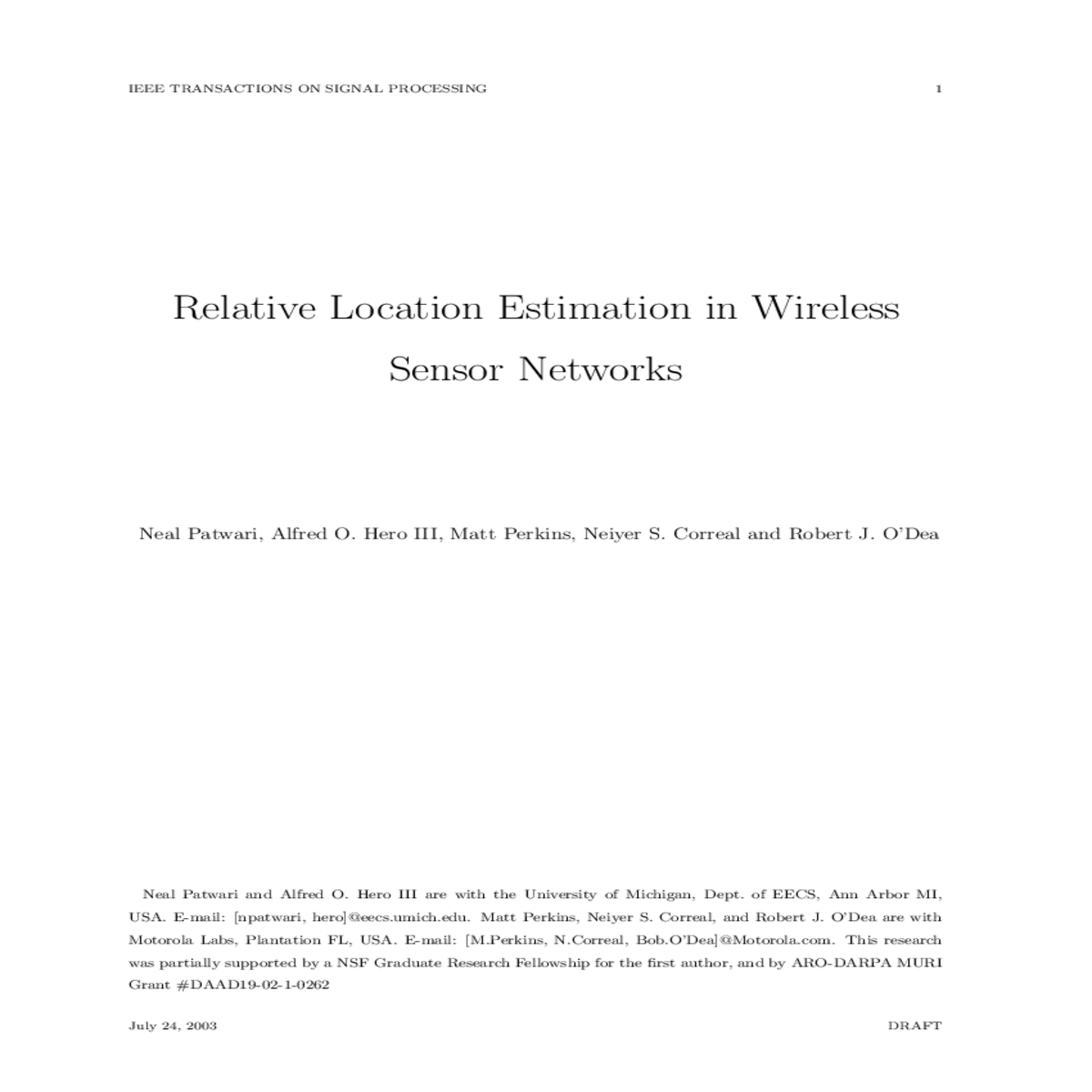
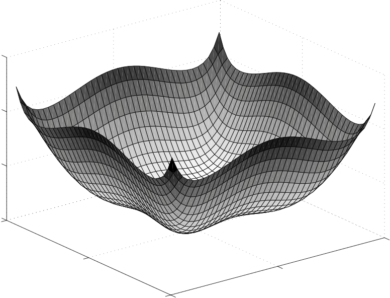
However, there remains residual bias. Consider m = 4 and n = 1. Place the reference devices at the corners of a 1 m by 1 m square and the blindfolded device within the square, the same as the case plotted in Fig. 1. We calculate via simulation [22] the bias gradient norm of ˆx1 given by (16) and display it in Fig. 2.
The gradient of the bias can be used in the uniform CRB to calculate
the achievable variance of the biased estimator [22] as compared to all
other estimators with same or less bias gradi-ent norm. Fig. 2 shows
that the bias gradient is high (with norm ≈1) at the corners of
the 1,j/(C2d2 1,j) close to 1. If
square. Expression (16) shows that the MLE tries to force the ratio
˜d2
the blindfolded device is very close to one reference device and far
away from the others, then measurements from the other three reference
devices provide relatively little information regard-ing the placement
of the blindfolded device. In the limit as the blindfolded device
approaches a reference device, it can only be localized to a circle
around that reference. Thus no unbiased estimator is possible. The MLE
in (16) approaches a constant in the limit, and thus the bias gradient
norm approaches 1.
IEEE TRANSACTIONS ON SIGNAL PROCESSING 12
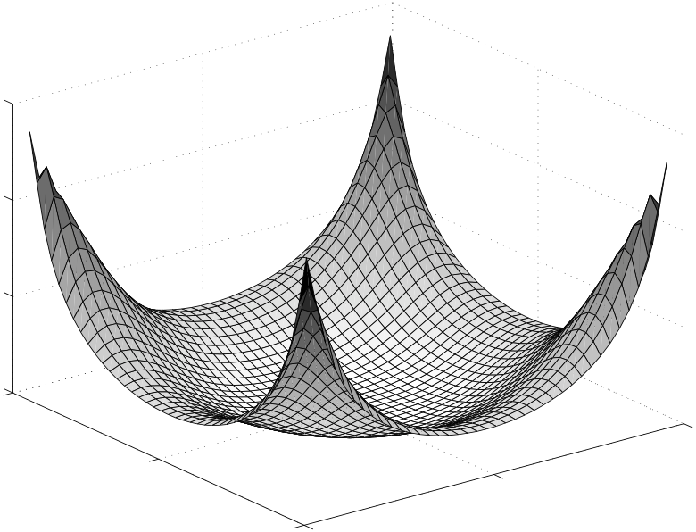
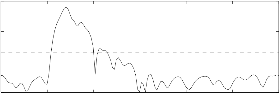
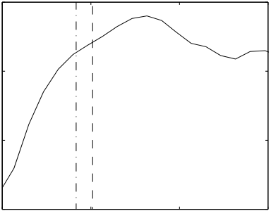
The measurement system uses a wideband direct-sequence spread-spectrum (DS-SS) transmit-ter (TX) and receiver (RX) (Sigtek model ST-515). The TX and RX are battery-powered and are placed on carts. The TX outputs an unmodulated pseudo-noise (PN) code signal with a 40 MHz chip rate and code length 1024. The center frequency is 2443 MHz, and the transmit power is 10 mW. Both TX and RX use 2.4 GHz sleeve dipole antennas kept 1m above the floor. The antennas have an omnidirectional pattern in the horizontal plane and a measured antenna gain of 1.1 dBi. The RX records I and Q samples at a rate of 120 MHz, downconverts, and correlates them with the known PN signal and outputs a power-delay profile (PDP). An example PDP is shown in Fig. 4. We ensure that noise and ISM-band interference is not an issue by maintaining an SNR > 25 dB throughout the campaign.

Fig. 3. Photo of measurement area looking above cubicle walls.
July 24, 2003 DRAFT
−100
−120
−120
0.5
0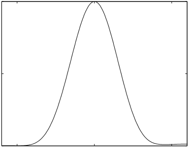
Fig. 4. (a) Measured PDP with TX at 1 and RX at 24 and threshold (- - -) above which received power is
integrated to calculate RSS. (b) Leading edge of same PDP showing LOS TOA = d1,24/c (· −· −·) and estimated
than 2/RC. However, a wider peak permits more multipath errors since the line-of-sight (LOS)
component, with TOA di,j/c, can be obscured by non-LOS multipath that arrive < 2/RC seconds
The template-matching method [23] provides a TOA estimation algorithm which is robust to
such attenuated-LOS multipath channels. In template-matching, samples of the leading edge of
been much greater.
Since non-LOS multipath are delayed in time, ˜ti,j usually has a positive bias. We estimate the
−60
−70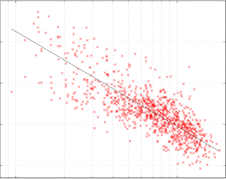
Fig. 5. Measured wideband path gain (x) as a function of path length. Linear fit (—) is with d0 = 1m, np = 2.3,
and σdB = 3.92.
| Fig. 6. |
|
|
|---|---|---|
|
|
|
| Q-Q plot of (a) Pi,j(dBm) −¯Pi,j(dBm) for RSS data, and (b) Ti,j −di,j/c for TOA data, compared to a | ||
we get the unbiased TOA estimator ti,j. Finally, the average of the 10 ti,j measurements for the
link between i and j we call Ti,j. The measured standard deviation, σT , is 6.1 ns.
IEEE TRANSACTIONS ON SIGNAL PROCESSING 16
reduces the frequency-selective fading effects. The geometric mean of the 10 pi,j measurements for the link between i and j, which we call Pi,j, reduces fading due to motion of objects in the channel. Shadowing effects, caused by permanent obstructions in the channel, remain pre-dominant in Pi,j since the TX and RX are stationary. Shadowing loss is often reported to be a log-normal random variable [24][18][21], which lead us to propose the log-normal shadowing model in (6). As shown in Fig. 5, The measured Pi,j match the log-normal shadowing model in (6) with n = 2.30 and σdB = 3.92 dB, using d0 = 1m. The low variance may be due to the wide bandwidth, averaging, and homogeneity of the measured cubicle area.
July 24, 2003 DRAFT
IEEE TRANSACTIONS ON SIGNAL PROCESSING 17
First, we use the testbed as an easy way to estimate the path loss exponent np. When all of the device locations are known, the laptop uses the path loss vs. path length data to estimate the path loss exponent, np [25]. After estimating np, the blindfolded device coordinates are removed from the laptop and we operate the relative location estimation algorithm using the estimated np.
July 24, 2003 DRAFT
| IEEE TRANSACTIONS ON SIGNAL PROCESSING | 18 | ||||||
|---|---|---|---|---|---|---|---|
| (m) | 1T | 2E |
32T 31T |
||||
| 12 | |||||||
| 2T | |||||||
| 4E | |||||||
| 10 | |||||||
| 1E | 7E | 5T |
|
||||
| 7T | |||||||
| 8 | |||||||
| 6T | 6E | ||||||
| 6 | |||||||
| 8T | |||||||
| 4 | |||||||
| 2 | 10 | 9E 9T | |||||
| 0 | 11T | ||||||
| Fig. 7. | −2 | 11E | |||||||||||
|---|---|---|---|---|---|---|---|---|---|---|---|---|---|
| −4 | 0 | 2 | 4 | 6 | 8 | 10 | (m) | ||||||
| (m) | 1T | 3 |
36T
40E
|
||||||||||
| 12 | |||||||||||||
| 10 | 1E | 7E | 5T | ||||||||||
| 8 | 7T | ||||||||||||
| 5E | |||||||||||||
| 6T | 6E | ||||||||||||
| 6 | 8T | 8E | |||||||||||
| 4 | |||||||||||||
| 2 |
|
||||||||||||
| 0 | 11E | ||||||||||||
| 11T | |||||||||||||
| −4 | 0 | 2 | 4 | 6 | 8 | 10 | |||||||
| True (•#T) and estimated (H#E) location using (a) RSS and (b) TOA data for measured network with | |||||||||||||
IEEE TRANSACTIONS ON SIGNAL PROCESSING 19
Next, the relative location estimation algorithm averages the measurements over time (using the most recent four RSS measurements), frequency (across 8 center frequencies), and the recip-rocal channel, resulting in the averaged measurement Pi,j. The maximum of the MLE in (16) is found using a conjugate gradient algorithm, which takes less than one second on the Pentium laptop. Each second an updated location is calculated and displayed on a map in a Visual Basic GUI. Real time tracking of slow movement (eg., people walking) is possible.
B. Residential Home
Next, we test the system in the Perkins home, a single-family, ranch-style house in Sunrise, Florida (Figs. 9 and 10). An identical 9 m by 9 m grid is used in this test, which spanned across
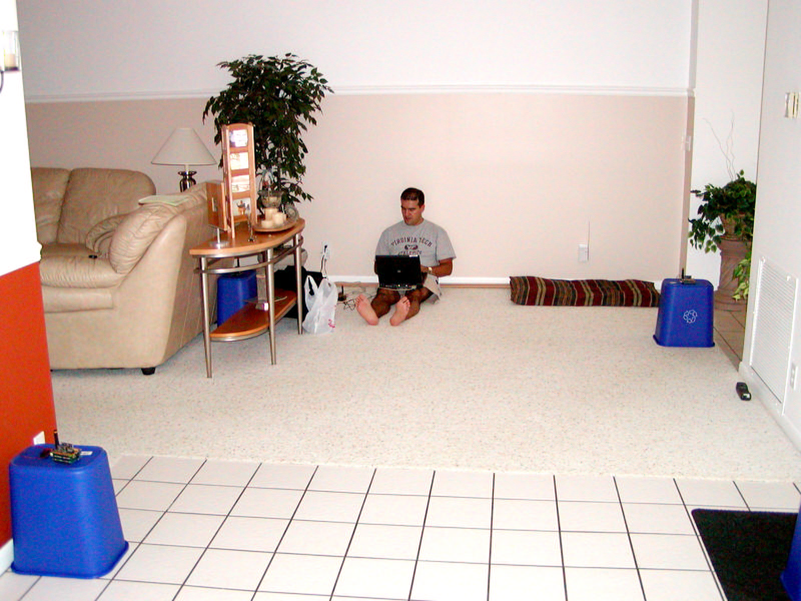
Fig. 10. Residential home testbed experiment, with 3 devices shown (one is hidden between the couch and the table).


