

And are the kinematic viscosity and thermal diffusivity
J. Fluid Mech. (2022), vol. 946, A6, doi:10.1017/jfm.2022.554

| 2.554 Published online by Cambridge University Press |
in addition to the filtered scale contributions associated with the processes of strain |
|
|---|---|---|
| https://doi.org/10.1017/jfm.202 | ||
| 946 A6-1 | ||
X. Zhang and others
1. Introduction
|
|---|
|
|---|
stratified turbulence across scales could aid in the development of appropriate sub-grid models.
and discuss areas for future investigation.
2. Theoretical considerations
| https://doi.org/10.1017/jfm.2022.554 Published online by Cambridge University Press |
946 A6-3 |
|---|
|
|---|
Energy source
(forcing)
| EK | ΠK | eK | B | eP | ΠP |
|
|---|---|---|---|---|---|---|
| ∇∙TP | ||||||
| ∇∙TK |
2.2. Length scales in SSST |
|---|
| Ri ≡N2 γ2 = (ℓC/ℓO)4/3, | (2.11) |
|---|---|
Reb ≡ ⟨ϵK⟩νN2 = (ℓO/η)4/3, |
(2.12) (2.13) |
| Res ≡ ⟨ϵK⟩νγ2 = (ℓC/η)4/3. | (2.14) |
|
||
|---|---|---|
|
||
| ⟨FK⟩∞∼ −⟨B⟩∞+ ⟨ϵK⟩, | (2.17) | |
|
||
Analysis of scale-dependent kinetic and potential energy
|
|---|
| ⟨ΠK⟩ ∼ −γ2⟨ϵK⟩1/3ℓ4/3+ ⟨ϵK⟩, | (2.18) | ||
|---|---|---|---|
|
|||
| (2.19) | |||
946 A6-7 |
|||
dimensions; however, the underlying mechanisms driving the energy transfers in HIT and SSST might be quite different. In the context of HIT, it has long been thought that the key mechanism driving the TKE cascade is that of vortex stretching (VS) (Taylor 1922, 1938; Tennekes & Lumley 1972; Davidson 2004; Doan et al. 2018). However, recent studies have demonstrated quantitatively that while VS plays an important role, the largest contribution to the TKE cascade comes from the dynamical process of the self-amplification of the strain-rate field (Carbone & Bragg 2020; Johnson 2020, 2021). An important question is how this understanding applies to SSST, where effects such as internal waves and mean-shear can play a role (whether directly or indirectly) in how TKE is transferred between scales, as well as the question of the mechanism driving the TPE transfer. In Johnson (2020, 2021), a powerful, exact relationship was derived for ΠK that assumes only that the filtering kernel Gℓ used in constructing ˜u is Gaussian. The result is
|
ΠK = ΠF,SSA | + ΠSG,C | , | (2.22) | |
|---|---|---|---|---|---|
| (2.23) | |||||
| (2.24) | |||||
|
|||||
|
|---|
| https://doi.org/10.1017/jfm.2022.554 Published online by Cambridge University Press |
|
|
|---|---|---|
ΠP = ΠF P+ ΠSG,S + ΠSG,V , |
(2.27) (2.28) |
|
|
|---|
| Reb | Ri | Res | Fr | L/η | ℓO/η | ℓC/η | |
|---|---|---|---|---|---|---|---|
| 160 | 0.157 | 25.12 | 0.48 | 126.35 | 43.90 | 10.36 |
of the TKE and TPE across scales in SSST. The DNS data used are from the data set presented in Portwood et al. (2019) and Portwood, de Bruyn Kops & Caulfield (2022), which we summarize here. In the DNS, the unfiltered versions of (2.1) and (2.2) are solved with constant mean velocity gradient γ and mean density gradient ζ using the Fourier pseudospectral scheme described in de Bruyn Kops (2015) and Almalkie & de Bruyn
|
|
|---|
X. Zhang and others
| (a) | 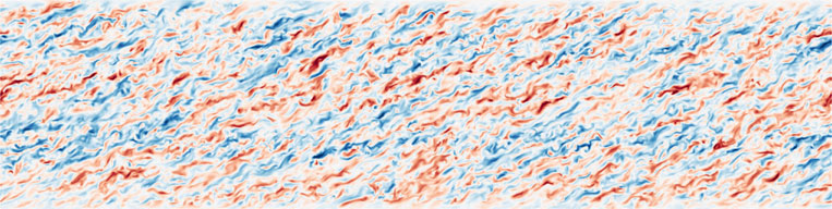 |
||
|---|---|---|---|
| (b) | 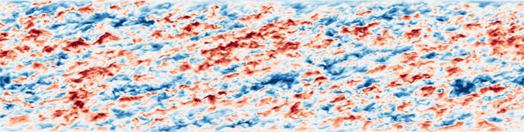 |
||
| (c) |  |
||
| (d ) | 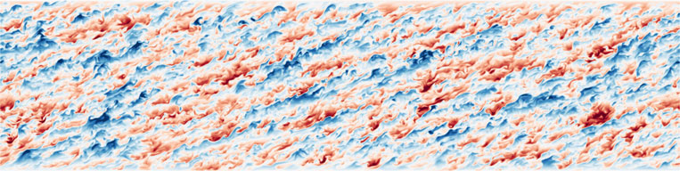 |
||
2EK/3, (d) fluctuating density ρ′/√⟨ρ′ρ′⟩. Values go from (red,�2EK/3, (b) streamwise component
|
|||
|
(a) | 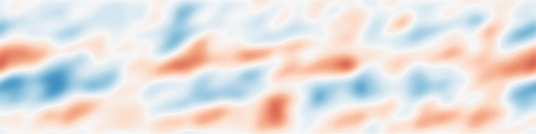 |
|
|---|---|---|---|
| (b) | 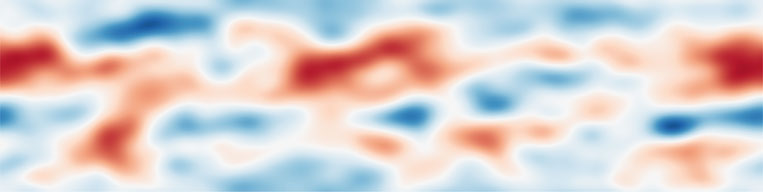 |
||
| (c) | |||
| (d ) | |||
|
|||

X. Zhang and others
| (a) | 100 | ⟨eK⟩/⟨ET⟩ | (b) | 100 | ⟨εK⟩/⟨ϵT⟩ | |||
|---|---|---|---|---|---|---|---|---|
| 100 | 100 | |||||||
| 10–1 | 10–1 | |||||||
| 10–2 | ⟨τxx⟩/[2⟨ET⟩] | 10–2 | ||||||
| 10–3 | ⟨εP⟩/⟨ϵT⟩ | |||||||
|
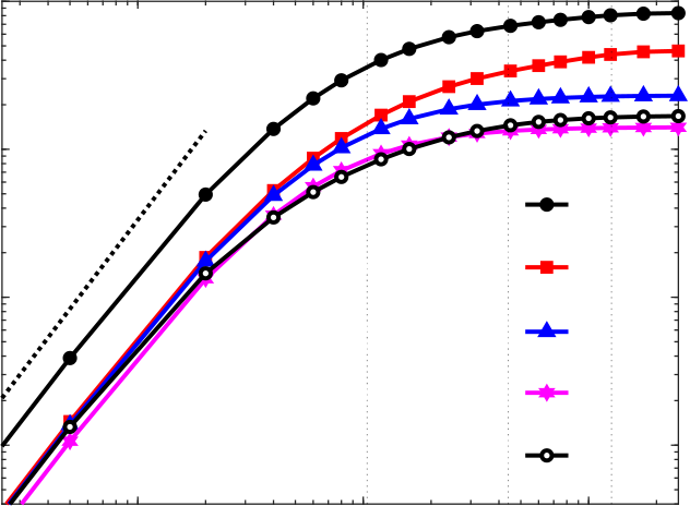
Figure 4. (a) Plot of mean small-scale TKE ⟨eK⟩, TPE ⟨eP⟩, and diagonal components of ⟨τ⟩/2, normalized by total energy ⟨ET⟩ ≡ limℓ/η→∞[⟨eK⟩ + ⟨eP⟩], as a function of filter scale ℓ. The thick dotted line indicates scaling ∝ ℓ2. (b) Plot of mean small-scale TKE ⟨εK⟩ and TPE ⟨εP⟩ dissipation rates, normalized by the total turbulent energy dissipation rate ⟨ϵT⟩ ≡ limℓ/η→∞[⟨εK⟩ + ⟨εP⟩]. The thin vertical dotted lines from right to left are L/η, ℓO/η, ℓC/η = 126.3, 43.9, 10.4, respectively.
|
|---|
| 100 | 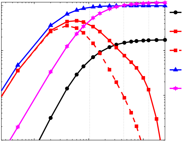 |
|||
|---|---|---|---|---|
| 10–1 |
|
|||
| 10–2 |
|
|||
| 10–3 | ||||
| 100 | 102 | |||
|
|---|
| 100 | 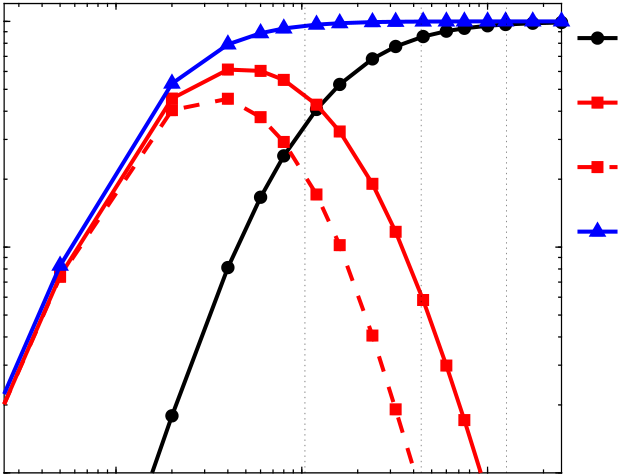 |
|||
|---|---|---|---|---|
| 10–1 |
|
|||
|
||||
| 10–2 | ||||
| 100 | 102 | |||
lengths ℓ/η. At larger scales, the PDFs have a large variance, showing that at these scales, In figure 7(c), we show the PDFs of ΠK/⟨ΠK⟩ and ΠP/⟨ΠP⟩ for different filtering
the fluxes of TKE and TPE can exceed their mean values significantly. The PDFs are also
|
|---|
| (a) | (b) | ||||||||||||||
|---|---|---|---|---|---|---|---|---|---|---|---|---|---|---|---|
| 100 | 1 |
|
|
5 | 100 | 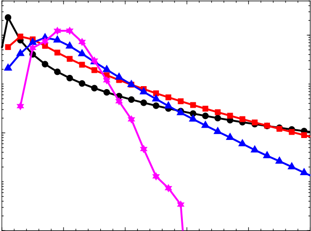 |
|||||||||
| 10–2 | 10–2 | ||||||||||||||
| 10–4 | 4 | 10–4 | |||||||||||||
|
1 |
|
4 | 5 | |||||||||||
| (c) | (d ) | ||||||||||||||
ΠK/⟨ΠK⟩, ΠP/⟨ΠP⟩ |
B/⟨B⟩ |
||||||||||||||
946 A6-17 |
|||||||||||||||
|
|||||||||||||||||||||
|---|---|---|---|---|---|---|---|---|---|---|---|---|---|---|---|---|---|---|---|---|---|
|
|||||||||||||||||||||
| 10 | |||||||||||||||||||||
| 0 | 100 | 101 |
|
||||||||||||||||||
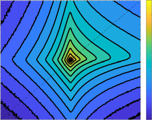
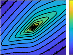
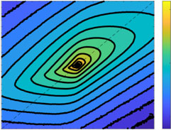
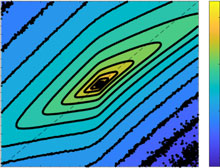
| (a) | 5 | Corr = 0.22695 | (b) | 5 | Corr = 0.1474 | ||||||||||||||||
 |
 |
||||||||||||||||||||
| 3 | 3 | ||||||||||||||||||||
|
|
||||||||||||||||||||
| 1 | |||||||||||||||||||||
|
–1 | ||||||||||||||||||||
|
|||||||||||||||||||||
| –3 | |||||||||||||||||||||
| –3 | |||||||||||||||||||||
| –10 | |||||||||||||||||||||
| –10 | |||||||||||||||||||||
| –12 | |||||||||||||||||||||
| –5 | –3 | –1 | 1 | 3 | 5 | –5 | –3 | –1 | 1 | 3 | 5 | ||||||||||
| (c) | 5 | Corr = 0.23027 | Corr = 0.14807 |
|
|||||||||||||||||
 |
 |
||||||||||||||||||||
| 3 |
|
3 | |||||||||||||||||||
| 1 |
|
||||||||||||||||||||
|
–1 | ||||||||||||||||||||
| –3 | –3 | ||||||||||||||||||||
| –5 | –10 | –5 |
|
||||||||||||||||||
| –3 | –1 | 1 | 3 | 5 | –3 | –1 | 1 | 3 | 5 | ||||||||||||
| ΠP/⟨ΠP⟩ | ΠP/⟨ΠP⟩ | ||||||||||||||||||||
|
|||||||||||||||||||||
|
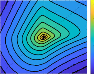
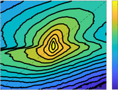
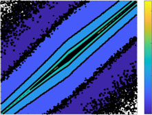
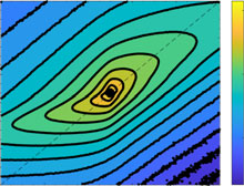
(a) | 5 | Corr = 0.99352 |
|
(b) | 5 | Corr = 0.74019 | ||||||||||||||
|---|---|---|---|---|---|---|---|---|---|---|---|---|---|---|---|---|---|---|---|---|---|
 |
 |
||||||||||||||||||||
| 3 | 3 | ||||||||||||||||||||
| 1 |
|
||||||||||||||||||||
| –10 | –1 | ||||||||||||||||||||
| –3 | –15 | –3 |
|
||||||||||||||||||
| –5 | –3 | –1 | 1 | 3 | 5 | –5 | –3 | –1 | 1 | 3 | 5 | ||||||||||
| (c) | Corr = 0.55206 | 5 | Corr = 0.32478 | ||||||||||||||||||
| 5 | |||||||||||||||||||||
 |
 |
||||||||||||||||||||
| 3 | 3 |
|
|||||||||||||||||||
|
|||||||||||||||||||||
| 1 | |||||||||||||||||||||
| –1 | |||||||||||||||||||||
| –3 | –10 | –3 | |||||||||||||||||||
| –5 | –3 | –1 | 1 | 3 | 5 | –5 | –3 | –1 | 1 | 3 |
|
||||||||||
| ΠK F /⟨ΠK F⟩ | ΠK F /⟨ΠK F⟩ | ||||||||||||||||||||
|
|||||||||||||||||||||
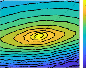
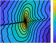
| (a) | 5 | Corr = 0.99554 | (b) | 5 | Corr = 0.80967 |
|
||||||||||
|---|---|---|---|---|---|---|---|---|---|---|---|---|---|---|---|---|
 |
 |
|||||||||||||||
| 3 | 3 | |||||||||||||||
|
1 | |||||||||||||||
| –10 | ||||||||||||||||
| –1 | ||||||||||||||||
| –3 | –15 | –3 |
|
|||||||||||||
| –5 | –3 | –1 | 1 | 3 | 5 | –5 | –3 | –1 | 1 | 3 |
|
|||||
| (c) | 5 | Corr = 0.65245 | Corr = 0.287 | |||||||||||||
 |
 |
|||||||||||||||
| 3 | 3 | |||||||||||||||
–1 |
|
1 | ||||||||||||||
| –1 | ||||||||||||||||
| –10 | –3 | |||||||||||||||
| –3 | ||||||||||||||||
| –5 | –3 | –1 | 1 | 3 | 5 | –5 | –3 | –1 | 1 | 3 | ||||||
| ΠP F /⟨ΠP F⟩ | ||||||||||||||||
|
||||||||||||||||


