IS LM BP model
Mundell-Fleming model, also known as IS-LM BP model (or IS-LM BOP model) is an extension of the IS-LM model. This is an economic model which was formulated by economists Robert Mundell and Marcus Fleming. While IS-LM model dealt with goods and asset markets in a closed economy (or autarky), Mundell-Fleming model is a version of IS-LM which deals with the interaction of goods and asset markets in an open economy.
Economies of the world are related to one another internationally through trade in goods and through financial markets. In addition to studying equilibrium in goods and money markets (as done by IS-LM model), the model also carries out analysis on the balance of payments.
In order to understand the working of the Mundell-Fleming model, we need to first understand the concepts of IS curve (which represents the goods market equilibrium), LM curve (which represents money market equilibrium) and BP curve (which represents equilibrium of the balance of payments).
IS CURVE: EQUILIBRIUM IN GOODS MARKET
IS curve (or schedule) shows the combinations of interest rates and level of real output such that planned spending equals income. IS curve is also known as goods market equilibrium schedule.
In an open economy, equilibrium in goods market is achieved when production or income (Y) is equal to Aggregate demand (AD) which is the sum of consumption, planned investment spending, government spending and net exports (exports-imports). The equilibrium equation is given as:
Y=AD
Y=C+I+G+NE
Where C= consumption
I=planned investment spending
G= Government spending
NE= net exports
In the model, planned investment spending is not constant i.e. it is not autonomous but depends on the level of sales and the interest rates. If sales of firm increases, this is a reflection of an increase in the demand for the goods of the firm and thus the firm will have to invest in the necessary plant and machinery in order to raise the production level. Thus, there is a positive relationship between investment and level of sales. However, there is a negative relationship between the level of investment in an economy and interest rates, higher the interest rates, higher is the cost of borrowing funds for the firm in order to undertake investment. In other words, an increase in interest rates decreases the profitability of adding to the capital stock and therefore leads to higher planned investment spending in the economy.
Consumption is a function of disposable income i.e. C(Y-T) where T is the taxes.
Net exports are a function of real exchange rates (e), foreign income (Yf) and domestic income (Y). Thus, the level of competitiveness as measured by real exchange rates affects the open economy IS curve. Net exports are also affected by the level of foreign income (Yf). An increase in foreign income may lead to increase in foreign spending on domestic goods will increase net export or demand for domestic goods.
An increase in domestic income will increase the demand of both, domestic goods and foreign goods. This leads to increase in imports and thus worsening of trade balance (NX=X-M).
Therefore, the equilibrium relationship can be expressed as:
Y= C(Y-T) + I (Y, i) + G + NE (e, Yf, Y)
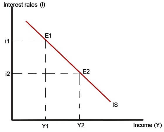
The above figure shows a downward sloping IS a curve, expressing a negative relationship between income (on X-axis) and interest rates (on the Y-axis). At each interest rate (i1 and i2), the goods market is in equilibrium (production=demand).
Suppose that initially, the goods and services market is in equilibrium at point E1 with equilibrium output being Y1 and equilibrium level of the interest rate being i1. Now let the interest rate decrease. As the interest rate decreases, the profitability of investment increases due to a decrease in borrowing costs. This leads to an increase in planned investment spending in the economy. Now, as planned investment is a part of aggregate demand, increase in investment spending also causes an increase in Aggregate demand. This leads to increase in production (in order to meet higher aggregate demand) and as a result income (or output) shifts from Y1 to Y2 and a new equilibrium is achieved at point E2.
LM CURVE: MONEY MARKET EQUILIBRIUM
LM curve (or schedule) shows the combinations of interest rates and level of output such that demand for money equals the supply of money. LM curve is also known as money market equilibrium schedule.
Demand for money: Demand for money is the demand for real balance because people hold money for what it will buy. Real money balance is the quantity of nominal money (M) divided by price index (P) i.e.(M/P). Higher the price level in an economy, more quantity of nominal money is required in order to buy the same amount of goods. Demand for real balances (M/P) is a function of the level of income (Y) and the interest rate (i) and is expressed as:
Demand of money=L (Y, i)
Demand for real money balances depends on real income level because any individual requires money in order to purchase goods and services, which in turn depends upon the level of his real income (which tells about the purchasing power of an individual).
The cost of holding is the interest rate that is foregone by holding money rather than any interest-bearing asset such as bonds. When interest rates rise, the cost of holding money rises and as a result demand for holding real money balance falls at each level of income. In this case, People transfer their cash holdings to assets such as bonds.
Thus, the demand for real balances is positively related to the level of income and negatively related to the interest rates.
Supply of money: The supply of money (nominal quantity of money, M) is controlled by the central bank in any country and is thus taken to be as given, M ̅. It is assumed that the price level is constant at P̅. So, we say that the real money supply in the economy is fixed at( M̅/P̅).
The equilibrium in money market is determined when (M̅/P̅) = L (Y, i)
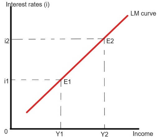
The figure below shows an upward sloping LM curve, expressing a positive relation between income (on X-axis) and interest rates (on the Y-axis). At each level of interest rate (i1 and i2), the money market is in equilibrium (Demand for money = supply of money).
When interest rate rises from i1 to i2, then the demand for money reduces due to increasing in the cost of borrowing. But the supply of money is given (decided by the central bank). So, to maintain the money market equilibrium, the level of real income has to rise until the opposite effect on the demand for money is canceled. People will demand less money due to increase in interest rates and more money when real income rises (from Y1 to Y2).
Capital Mobility
Capital mobility refers to the ability of private funds to move across national borders in quest of higher returns. The ease with which funds can be moved between economies depends on the restrictions (or obstacles) on inflow or outflow of funds put up by countries.
Perfect Capital Mobility
A capital is perfectly mobile internationally when an investor can purchase assets in any country quickly, with low transaction costs, and in unlimited amounts. When the capital is mobile, investors can invest freely (without any restrictions) by investing a large amount of funds with low cost of borrowing and highest possible return.
Example: Suppose there are only two countries in the world, A and B. There is perfect mobility of capital given the price of imports and export demand for the two countries. Now when there are differences in interest rates of the two countries such that A offers a higher interest rate on investment than B. This will result in higher capital inflows into the country A and outflows from country B as investors in quest of higher returns move funds from B to A.
Balance of Payment Curve (BP curve)
From above example of capital mobility, we can clearly infer that when there are perfect capital mobility and interest rates in the home country (i) is higher than world interest rate (if), then capital will flow into the home country at an unlimited rate. The converse happens when home country’s interest rates are below world interest rate (i.e. i<if). The slightest difference in interest rates will result in infinite capital flows.
The balance of payments surplus, BP, is equal to the sum of trade surplus (NX) and net capital inflows (capital account surplus), CF.
BP= NX + CF
Net capital flow depends on the interest differential (i.e. i-if). An increase in the domestic interest rate above the world interest rate (i>if) will result in net capital inflows from abroad and thus will improve capital account (a surplus in Capital account).
As discussed above IS curve section, NX depends on foreign income (Yf), domestic income (Y), and real exchange rate (e).
An increase in domestic income will result in higher exports (X) than imports (M) which will worsen the trade balance. On the other hand, an increase in domestic interest rate will result in higher capital flows into the domestic country from abroad (assuming perfectly mobility of capital).
Thus, we can say that when income increases, even a small increase in domestic interest rate (i) will maintain the overall balance of payments equilibrium. This means that a deficit in trade balance (higher imports than exports) will be viably financed by net capital inflows such that BP=0 at equilibrium (i.e. deficit in trade balance = net capital flows).
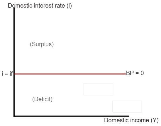
The BP curve is flat due to perfect capital mobility. The slope of BP curve is determined by the degree of capital mobility possible. When imports are higher, then the balance of payment will be in the deficit unless domestic interest rate rises to maintain the equilibrium (high-interest rates will lead to capital inflows which will finance the trade deficit). Higher the mobility of capital, flatter will be the BP curve.
Any point above the BP curve means that Balance of payments (BOP) is in surplus (BOP>0) while all the point below the BP curve means that the BOP is in deficit (BOP<0).
The Mundell-Fleming Model with Perfect Capital Mobility
PERFECT MOBILITY OF CAPITAL UNDER FIXED EXCHANGE RATE
FIXED EXCHANGE RATE: Fixed exchange rate system is an exchange rate regime in which currency’s value is fixed against either the value of another single currency or to a basket of other currencies, or to another measure of value, such as gold.
This type of exchange rate is not determined by market forces of demand and supply.
In all the analysis carried below, we assume that the economy initially is in equilibrium and the domestic interest rates (i) and world interest rates (if) are same. The balance of payment is initially in equilibrium (BP=0).
(A) Expansionary monetary policy in case of Mundell-Fleming Model with Fixed Exchange Rate and Perfect Capital Mobility
An expansionary monetary policy will shift the LM curve from LM1 to LM2. This shifts the equilibrium point to shift from E to E’. Now we see that the point E’ is below the BP curve. This means that the economy has a balance of payment deficit. The domestic interest rates are below the world interest rate (iif). This leads to capital outflows in the domestic countries. The foreign investors try to sell the domestic assets, tending to cause a depreciation in the exchange rate. Now as the economy follows a fixed exchange rate system, the central bank has to intervene to hold the exchange rate constant. The central bank sells foreign currency and buys domestic currency. This intervention results in lower money supply in the domestic economy thus shifting the LM curve from LM2 to LM1(original LM curve). Clearly, the initial monetary expansion is reversed and the process ends when the domestic interest rates are back to the initial level (where i=if).
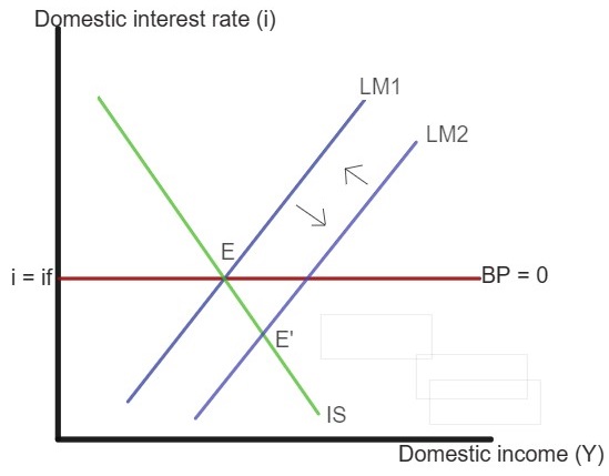
Thus, under fixed exchange rate system and perfect capital mobility, a country cannot take up independent monetary policy. Interest rates cannot move out of the line with those prevailing in the world market (if).
(B) Expansionary fiscal policy in case of Mundell-Fleming Model with Fixed Exchange Rate and Perfect Capital Mobility
An expansionary fiscal policy shifts the IS curve from IS1 to IS2. This shifts the equilibrium point from E to E’. Now we see that the point E’ is above the BP curve. This means that the economy has a balance of payment surplus. The domestic interest rates are above the world interest rate (i > if). This leads to capital inflows in the domestic country. The foreign investors try to buy the domestic assets, tending to cause an appreciation in the exchange rate.
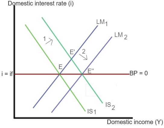
Now as the economy follows a fixed exchange rate system, the central bank has to intervene to hold the exchange rate constant. The central bank buys foreign currency and sells domestic currency. This intervention results in higher money supply in the domestic economy thus shifting the LM curve from LM1 to LM2 which increases the income further. The equilibrium (E”) is achieved when the money supply has increased enough to drive the domestic interest rates back to the initial level (where, i=if).
PERFECT CAPITAL MOBILITY UNDER FLEXIBLE EXCHANGE RATE
FLEXIBLE EXCHANGE RATE: Flexible exchange rate or floating exchange rate is a type of exchange rate regime that allows the exchange rate to be determined by the forces of demand and supply. Under this system, the central bank does not intervene in the market for foreign exchange.
(A) Expansionary monetary policy in case of Mundell-Fleming Model with Flexible Exchange Rate and Perfect Capital Mobility
An expansionary monetary policy shifts the LM curve from LM1 to LM2. This shifts the equilibrium point from E to E’. Now we see that the point E’ is below the BP curve. This means that the economy has a balance of payment deficit. The domestic interest rates are below the world interest rate (i < if). This leads to capital outflows in the domestic country.
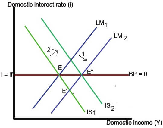
The foreign investors try to sell the domestic assets. Now as the economy follows a flexible exchange rate system, the central bank will not intervene to hold the exchange rate constant. As a result, the deficit in BOP causes the domestic currency to depreciate. This will increase the foreign demand for domestic goods as foreigners can buy more goods for the same amount. This shifts the IS curve from IS1 to IS2. As a result, income increases further. The equilibrium (E”) is achieved when an increase in foreign demand for domestic goods is enough to drive the domestic interest rates back to the initial level (where, i=if).
(B) Expansionary fiscal policy in case of Mundell-Fleming Model with Flexible Exchange Rate and Perfect Capital Mobility
An expansionary fiscal policy (higher government spending) shifts the IS curve from IS1 to IS2 (see figure). This shifts the equilibrium point from E to E’. Now we see that the point E’ is above the BP curve. This means that the economy has a balance of payment surplus.
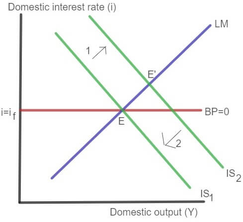
The domestic interest rates are above the world interest rate (i>if). This leads to capital inflows in the domestic country. The foreign investors try to buy the domestic assets. Now as the economy follows a flexible exchange rate system, the central bank will not intervene to hold the exchange rate constant. As a result, the surplus in BOP causes the domestic currency to appreciate. This will increase the domestic demand for foreign goods i.e. imports will rise as people in the domestic country can buy more goods for less money. Exports reduce as foreign demand for domestic good reduces. As a result, overall Net exports register a fall. This shifts the IS curve back from IS2 to IS1 (original IS curve). As a result, income increases further. The equilibrium (E”) is achieved when a decrease in foreign demand for domestic goods is enough to drive the domestic interest rates back to the initial level (where, i=if). the final equilibrium corresponds to initial equilibrium E.
Conclusion on Mundell-Fleming Model
The analysis carried above, under the assumption of perfect mobility of capital, monetary policy is completely ineffective in the case of fixed exchange rate. However, under flexible exchange rates, the central bank does not intervene in the foreign exchange market, and so the money stock increase in case of monetary expansion is not reversed leading to depreciation of the currency and increase in output. This states that monetary policy is effective in the case of flexible exchange rate system.
Fiscal policy, on the other hand, is effective in fixed exchange rate system but does not change the level of output (ineffective) in the case of flexible exchange rate system.
Online Macroeconomics Homework Help Tutors by Assignmenthelp
Macroeconomics is a vast subject area with a wide variety of topics such as GDP, Economics Growth Models, Keynesian Model total expenditure and total income, aggregate demand and aggregate supply, the balance of payment and much more. Under Macroeconomics as well as International Economics students have to study about the Mundell-Fleming Model of IS-LM-BP curves. This model can be very confusing for first-time readers as it has a variety of assumptions and macroeconomics model forms. Thus, it is best for students to study Mundell-Fleming model with a macroeconomics expert who can guide them in the best possible way to not only explain the model but also help students practice macroeconomic homework problems based on this model. At Assignment Help we boast of the best Macroeconomics homework help tutors for all areas under macroeconomics study and for all grades, whether it is for AP macroeconomics or it is intermediate level college macroeconomics study or even if it is advanced macroeconomic topics such as dynamic modelling for graduate research students of macroeconomics. At Assignment Help, we have the best macroeconomics tutors to help you with macroeconomics homework help, macroeconomics Assignment Help as well as macroeconomics research writing on relevant economics research topics.


