Consumer Behaviour
Consumer Behaviour
Choice, Utility and Preferences
Consumer behaviour theory tries to explain the relationship between price changes and consumer demand. Utility is a concept used to denote the subjective satisfaction or usefulness attained from consuming goods and services. This concept helps to explain how consumers divide their limited income / resources among different choices of goods and services that help attain them satisfaction (utility). The issue however is how we are supposed to measure utility and how the value of utility derived from various choices can be quantified. Because of these issues, the consumer behaviour theory has been reformulated and utility is viewed as a way to describe preferences. It was recognised that all that mattered about utility is whether one combination of choice had a higher utility than another; by how much higher or lower didn't really matter
Preferences of consumers is the fundamental description important for analyzing choice while utility is just a simple way of describing preferences
Total utility
The total satisfaction or fulfilment received by a consumer through the consumption of a goods or services or a combination of both is defined as Total utility. For instance if a person consumes five units of a commodity and derives U1, U2, U3, U4, U5 utility from the successive units of a good, his total utility will be,
TU = U1+ U2 +U3+ U4+ U5
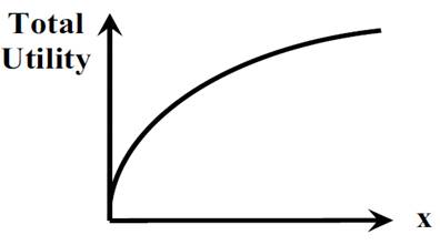
Total utility increases with an increase in consumption, but as consumption rises, total utility grows at a diminishing rate.
Every unit of a good or service has a marginal utility and the total utility is a simple addition of all the marginal utilities of the units of goods or services
All consumers want to achieve the maximum possible total utility for their spending and thus they look to combine different bundles of goods and services. With their limited resources, consumers make various choices in order to increase their total utility with each additional unit of consumption.

Marginal utility
As discussed above all consumers attempt to maximize their total utility from the goods and services they consume. This process of optimisation leads the consumers to consider the marginal utility of acquiring additional units of the product or service and of acquiring one product or service as opposed to another. Product characteristics and individual tastes and preferences apart from available resources (money) determine direct demand. Utility is maximised when products are bought at levels such that relative prices equal the relative marginal utility derived from consumption.
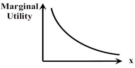
The marginal utility of a good is the increase in total utility gained by consuming one additional unit of that good, for a given level of consumption of other goods
Law of diminishing marginal utility
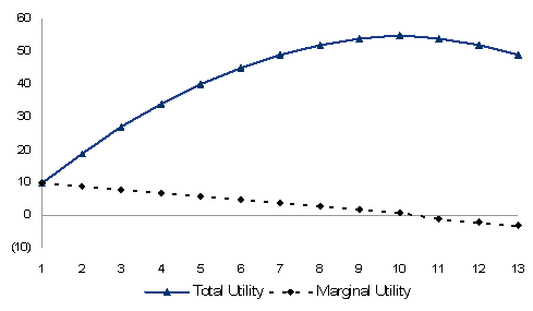
We have discussed earlier that with an increase in consumption total utility increases but at a slower and slower rate. Law of diminishing marginal utility explains this concept. The law of diminishing marginal utility says that as consumption rises the marginal utility of consuming the next unit is less than the previous one. Accordingly the marginal utility of good decreases as more and more units of that good are consumed as shown in the table and figure below:
| Quantity of Good | Total Utility (TU) | Marginal Utility (MU) |
| 1 | 10 | 10 |
| 2 | 19 | 9 |
| 3 | 27 | 8 |
| 4 | 34 | 7 |
| 5 | 40 | 6 |
Equimarginal Utility
The dollar value of a consumer's marginal utility from consuming additional unit of a product is called the marginal benefit. It is the maximum price that a consumer will pay for an additional unit and will fall as consumption increases. When different products are available a consumer will ensure that the last dollar spent on each product gives an equal marginal utility (MU) per dollar spent.
For two products A and B this can be expressed as:
![]() =
=![]()
MUA = marginal utility of product A;
MUB = marginal utility of product B
PA = price of product A;
PB = price of product B
To illustrate, let us take a case of a boy who wants to buy fruits and has $6 to spend. He finds that apples and oranges are available. While apples cost $2 per kilogram, oranges are available for $1 per kilogram. The marginal utilities of the first three kilograms of apples are $3, $2.50 and $2 respectively and the marginal utilities of the first 3 kilograms of oranges are $2.00, $1.25 and $1 respectively. The boy would achieve maximum utility by buying 2 kilograms of apples and 2 kilograms of oranges as the marginal utility of the last kilogram of each per dollar price is 1.25. In simpler words, if Apples cost costs twice as much as Oranges, then buy Apples only when the marginal utility derived from it is at least twice as great as Oranges' marginal utility.
Indifference Curve Analysis
As we know that the consumer is able to rank bundles of goods and services based on the utility he derives from them. This makes possible joining together of all these bundles that give the consumer equal utility / satisfaction. The curve drawn on these bundles or combinations of goods and services is known as indifference curve. At all points across the indifference curve the consumer derives same level of utility. And thus the consumers are indifferent because they do not care which of the bundles on the indifference curve they have.
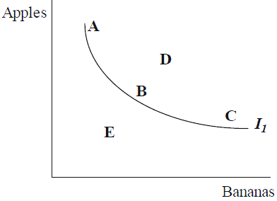
Compare the consumption bundles shown on the figure above. The indifference curve I1 tells us that Bundles A, B and C give the consumer equal satisfaction. Bundle E contains fewer bananas and fewer apples than Bundle B, and therefore Bundle B (and A and C) must be preferred to Bundle E. Similarly Bundle D contains more bananas and more apples than Bundle B, and therefore Bundle D must be preferred to Bundle B (and A and C). While bundle D should be on a higher indifference curves as it gives more utility to the consumer, E should be on a lower curves as it gives lesser utility. The indifference curves are convex to the origin as because to keep the consumers’ utility constant he must be compensated with increasingly larger amounts of good X for each additional unit of good Y he is giving up. This concept stems from the fact of diminishing marginal utility and is explained below in Marginal rate of substitution Slope of an Indifference curve is given by:
Marginal Rate of Substitution = ![]()
where MUA and MUB are marginal utility derived from the last unit consumed of good A and B respectively
All of the points along an indifference curve represent combinations of goods / services that are equally satisfying to the consumer
Marginal Rate of Substitution
The amount of one unit of good that a consumer is prepared to forego for one extra unit of another good is known as the marginal rate of substitution. The marginal rate of substitution of good A for good B is the number of good A the consumer is willing to give up to gain another unit of good B without affecting total satisfaction. A diminishing marginal rate of substitution of good B for good A implies that the consumer is willing to give up diminishing quantities of good A to gain each additional good B. This means that if it takes, say, n extra units of good A to convince a consumer to give up one unit of good B, it will take more than another n extra good A to persuade her to give up yet another unit of good B. Suppose the following combinations of fruits give the consumer equal satisfaction:
| Apples | Oranges |
| 20 | 1 |
| 15 | 2 |
| 11 | 3 |
| 8 | 4 |
The marginal rate of substitution of oranges for apples falls from 5 to 4 to 3, showing that the consumer is more willing to give up apples for an additional orange when the consumer has a lot of them.
Budget Constraint
The bundle of goods and services that the consumer can afford depends on two factors namely;
- Price of the goods; and
- Income of the consumer
Further to ascertain the bundles affordable by the consumer we assume that both the above factors are fixed which implies that the two factors are independent of the choice of consumption bundle
The budget line thus is a line drawn on all points that is affordable to the consumer, assuming that all income is spend
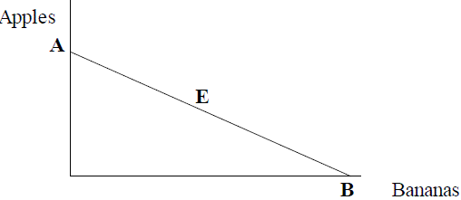
As shown in figure above, with a given income and prices of goods, if a consumer spends all his income on apples, he or she can afford to buy A apples. Alternatively, the consumer could buy B bananas, or an intermediate bundle such as E.
Consumer Equilibrium
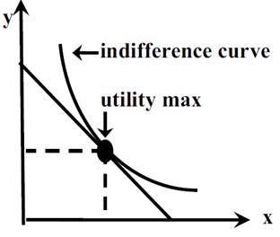
Individuals (consumers in this case) make their choices about the quantity of goods and services to be consumed with the objective to maximize their total utility. But in maximizing total utility they face several constraints, the foremost being the individual’s income level and the prices of the goods and services that he desires to consume. These constraints as discussed above forms the budget line of the consumer. The consumer's effort to maximize total utility, subject to the budget line, includes decisions about how much he would consume of the goods and services and the combination of goods and services at which the consumer maximises its total utility is called consumer equilibrium.
A consumer facing the budget line (fixed income and given market prices of goods) can come to a point (or equilibrium) of maximum satisfaction or utility only by acting in the following manner.
Each product is demanded up to the point where the marginal utility for every unit of money spent on it is exactly the same as the marginal utility of the spent on any other good. This fundamental condition of consumer equilibrium can be written in terms of Marginal Utilities (MU) and Prices (P) of the different goods in the following compact way.
![]() =
= ![]() =
= ![]() = Common MU per unit of income.
= Common MU per unit of income.
To maximise utility the consumers spread out their expenditures in such a way that the marginal rate of substitution is equal to the relative price of the good X as in the figure above. To represent it numerically:
![]() =
= ![]()
Thus combining the budget line with indifference curves, we can ascertain the consumption bundle which a consumer will choose. To further illustrate consider the earlier example of choice between apples and bananas and the figure below:
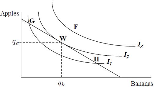
Now let assume that all income is spent. Since the bundle W lies on the highest achievable indifference curve, W will be chosen. At this point the consumer chooses to buy qa apples and qb bananas. Bundle F is unaffordable as it doesn’t touch the budget line and lies above it. Now though bundles such as G and H are affordable, but as they lie on a lower indifference curve and provide lower utility they will not be chosen. The bundle W maximises the consumer’s utility given the budget line and indifference curves.
Income and Substitution effect
If the price of a good increase whiles everything remaining same, the budget line rotates around the other good thus bringing down the consumer to a lower indifference curve
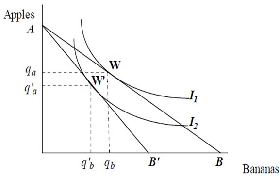
As shown in the figure above, when the price of bananas rises, the consumer can buy less of them though if he chooses to spend all his income on apples, he could buy just as many apples as before. So the budget line will rotate around A from AB to AB' and the consumer’s consumption bundle will change from W to W'. As seen here, the rise in the price of bananas has led the consumption of bananas to fall from qb to q′b. This change in the consumption bundle of the goods chosen by the consumer can be divided into two effects:
- Firstly, bananas become relatively more expensive compared with apples, and so $1 spent on bananas is less effective at increasing utility than $1 spent on apples. The consumer will therefore tend to substitute apples for bananas to some extent.
- Secondly, the increase in the price of bananas has made the consumer worse off by reducing his/ her real income as the consumer can buy less in total when the price of one good increases.
Substitution Effect
The substitution effect of the price change is the change in demand for the good/ services caused by the change in relative prices, holding the level of real income or utility of consumers constant.
Income Effect
The income effect of the price change is the change in demand for the good caused by the change in the real income of consumers as the price of a good change.
Analysing Substitution effect and Income Effect
The income and substitution effects can be separated and analysed by drawing a hypothetical budget line which has the slope of the new budget line and which is tangential to the old indifference curve. By using the old indifference curve we hypothetically keep real income constant thereby keeping the level of utility constant.
Refer the figure below:
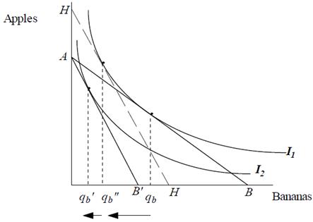
Continuing with our earlier illustration with the change in budget line with price rise we can analyse the income and substitution effects by drawing in the hypothetical budget line HH. This line reflects the new relative prices but the old level of utility (real income). Thus the difference between qb and q’’b is purely caused by the new relative prices. This is the substitution effect. The difference between q’’b and q’b is due to the change in real income as the relative prices are held constant. This is the income effect.
The shift from the old consumption bundle to the intermediate bundle with the same utility is the substitution effect
The income effect is the change from the intermediate bundle to the final bundle
Microeconomics Assignment Help | Microeconomics Help | Consumer Behaviour | Microeconomics Theories | principle of microeconomics | Economics course | Market Research On Consumer Behaviour | Concept of Consumer behaviour | behaviour Consumer | Online Tutoring


