The Phillips Curve shows

The Phillips curve: Relationship between inflation and unemployment

The Phillips curve concept was developed by A.W. Phillips in 1958. He gathered the data about the level of unemployment and the changes in wage levels in UK during late 19th century and thus he observed an inverse relationship between the two. The basis of the Phillips curve model is unemployment and inflation are inversely related or negatively related to each other i.e. when unemployment increases, inflation decreases and vice-versa. Here, in this model changes in wage levels are used as a proxy variable for inflation rate because wages are the largest component of prices. There exists a trade-off between unemployment and inflation. The theory states that with economic growth comes inflation, which in turn leads to more jobs and less unemployment.

The theory of the Phillips curve is known to be stable and predictable. Data from the 1960's modeled the trade-off between unemployment and inflation fairly well. The Phillips curve has potential economic policy outcomes on fiscal and monetary policies and they can be used to achieve full employment at the cost of higher price levels, or to lower inflation at the cost of lowered employment. The Phillips obtained from empirical evidences shows that it is a downward sloping curve.

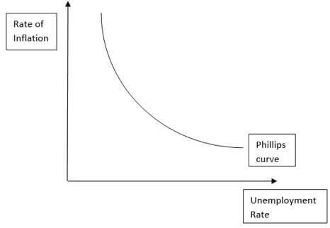
This inverse relation implies a trade-off, for reducing unemployment, price in the form of a higher rate of inflation will be the cost, and for reducing the rate of inflation, price in terms of a higher rate of unemployment has to be borne. Here, the horizontal axis shows the unemployment rate which is nothing but the share of labour force which is jobless; it is expressed in terms of percentage and the vertical axis measures inflation rate which is the rate of change of price level through a period of time. Empirical evidences from the developed countries also confirm the concept of Phillips curve. The graph below shows the inverse relationship between inflation and unemployment rates for United States during 1960s.

Explanation of the Shape of Phillip’s Curve Graph:

Keynesian economists assumed that Aggregate supply curve is upward sloping because of two main reasons; firstly, as the output of the firms in the economy increases, there exists diminishing returns to the factors like labour and thus there is a fall in the marginal physical product of labour (MPL). The amount of wage rate (W) is fixed and due to the fall in MPL, there will be a rise in the marginal cost (MC) of production as MC=W/MPL.

Secondly, under the pressure of aggregate demand for output, the demand for labour increases and this leads to a rise in wage rate and again shifts the MC.

Due to the above two reasons, the aggregate supply curve is upward sloping. Also, here the wage rate is used as a proxy variable for the inflation rate.

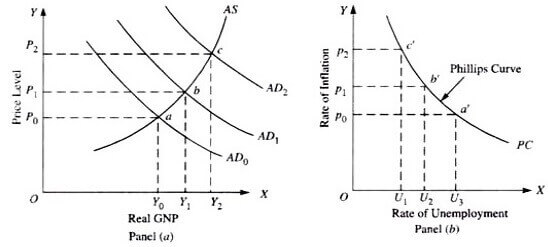
In the figure, the horizontal axis shows the output and the vertical axis shows the price level. Here, the economy is operating at the AD-0 and equilibrium is at point “a” with output Y-0 and price level P-0. When the economy expands and firms produce more, the aggregate demand increases to AD-1 and now the equilibrium shifted to point “b” and due to this there is an increase in the price level from P-0 TO P-1. So, an increase in the aggregate national output means the increase in employment because when aggregate demand increases, there is a demand for more goods and services and this leads to demand for more labour, due to this firms will hire more people resulting in more employment which means decrease in the unemployment rate.

Labor demand increases leading to decrease in the pool of unemployed workers and this makes the companies increase wages to compete and attract a smaller talent pool. The corporate cost of wages increases and companies pass along those costs to consumers in the form of higher price level.

This is reflected the second figure, when the economy was at point-a, it was at point-a’ on the Phillips curve and when the economy moved to point-b then it resulted in a change in the tradeoff levels in the Phillips curve because now the new point on Phillips curve was point-b’. And comparing points a’ with b’ it can be seen that point-b’ has higher price level and lower unemployment than point-a’. Thus, with an expanding economy we get higher inflation but lower unemployment rates and vice-versa; this is reflected in the second figure through which we derived the Phillips curve.

Through the increase in aggregate demand and upward-sloping aggregate supply curve, Keynesians explained the downward-sloping Phillips curve which reflects the negative relation between rates inflation and unemployment.

Collapse of Phillip’s Curve (1971-1991):

During the sixties Phillips curve concept became important for macroeconomic analysis. The stable relationship suggested that policy makers could have a lower rate of unemployment only at the cost of a higher rate of inflation and vice-versa. However, a stable Phillips curve did not hold good during the seventies and eighties, especially in the United States. The downward sloping Phillips curve nearly disappeared. This period raised the question of validity of the Phillips curve.

In these two decades, there were periods of both high rates of both inflation and unemployment. There is an absence of trade-off between inflation and unemployment. The Phillips curve kept shifting to the right. This period lead to stagflation. Stagflation occurs when an economy experiences stagnant economic growth with higher rates of unemployment and inflation. Stagflation was never experienced in the United States until the 1970s, when rising unemployment did not coincide with decreasing inflation and this was depicted on the Phillips curve and lead to its collapse.

Causes of Shift in Phillip’s curve:

Mainly there are two reasons for the shift in the Phillips curve. Firstly, Keynesians argued that higher inflation corresponding to higher unemployment was due the adverse supply shocks in the 1970s and 1980s which was from the increase in prices of oil and petroleum products. The increase in prices of oil by OPEC leads to a rise in the cost of production of several commodities which used oil as an input. The oil price hike raised the transportation costs of all commodities as well.

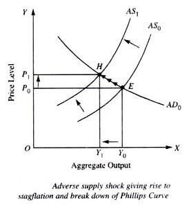
Suppose the economy is at point E with aggregate output Y-0 and price level P-0. Due to the adverse supply shock, the cost of production increased leading to the shift of aggregate supply curve to the left to AS-1. And the new equilibrium point is point-H. However, point-H is associated with lower level of output and higher level of price. This is the phase where the trade-off between the inflation and unemployment is invalid and stagflation sets in which results in collapse of Phillips curve.

Secondly, Milton Friedman had opposing views for the Phillips curve and this lead to its shift. He challenged the concept of a downward-sloping Phillips curve and its stability too. He argued that the trade-off between the inflation and unemployment exists only in the short run and there is no stable trade-off in the long run; Phillips curve is stable in the short run and shifts leftwards or rightwards in the long run. This happens because in the long run, economy is stable at the natural rate of unemployment. It is that rate of unemployment at which the current number of unemployed is equal to the number of jobs available. These workers are unemployed due to frictional and structural reasons. Friedman said that the long run Phillips curve is vertical.

The Adaptive Expectations Theory

Another reason for shift in the short-run Phillips curve is that expectations about the future rate of inflation play. This theory was given by Friedman and popularly known as the theory of adaptive expectations according to which people from their expectations on the basis of previous and present rate of inflation, and change or adapt their expectations only when the actual inflation turns out to be different from their expected rate.

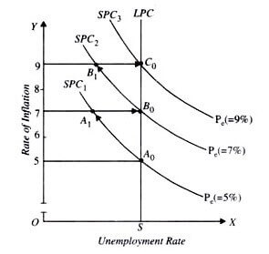
The horizontal axis represents the unemployment rate and the vertical axis represents the inflation rate. Suppose the economy is now at Phillips curve SPC-1 at A-0 with 5% inflation rate and S level of unemployment rate and this is at its natural level. People will thus make expectations about their nominal wages keeping in mind 5% inflation rate. Suppose the government adopts expansionary fiscal and monetary policies to increase aggregate demand. The increase in aggregate demand will raise the rate of inflation, say to 7%. Given the level of money wage rate being fixed on the basis that the 5% rate of inflation would continue to occur, the higher price level than expected would raise the profits of the firms which will induce the firms to increase their output and employ more labour; and due to these expansionary policies, unemployment decreases, therefore, the economy moves to point A-1 on the curve SPC-1. Here, the economy accepts a higher rate of inflation at the cost of lower unemployment.

Why is the Long Run Phillips Curve Vertical?

However, Friedman argued that the above phenomenon is temporary and the unemployment rate will return to its natural level in the long run. According to him, the economy will not remain in a stable equilibrium position at A-1 because the workers will realise that due to the higher rate of inflation than the expected one, their real wages and incomes have fallen. Thus, they will demand higher nominal wages to restore their real income. This will lead to fall in profits of the firms due to compensation of higher nominal wages. The reduction in profit means that the original motivation which encouraged them to expand output and increase employment resulting in lower unemployment rate will not exist anymore as it rises back to the natural level.

The increase is nominal wages will move the economy from A-1to B-0, at a higher inflation rate of 7%. The increase in aggregate demand raised the price level but due to the adaptive expectations of the people, the unemployment rate did not change. Thus, the short-run Phillips curves SPC shifts upward from SPC-1 to SPC-2. Thus, Friedman argued that the shift in Phillips curve is a temporary phenomenon but in the long run unemployment is at its natural level. This happens because; the nominal wages get fully adjusted to the changes in the inflation rate. This process may continue; an expansionary policy will just increase the price level and shift the short run Phillips curve upwards.

The Government may misjudge the situation and thinking 7% rate of inflation is too high and adopt expansionary fiscal and monetary policies to increase aggregate demand and thereby to expand the level of employment which again will raise the price level and nominal wages will lag behind in the short-run. Thus, the profits of business firms will increase and they will expand output and employment causing the reduction in rate of unemployment and rise in the inflation rate. When the workers will recognise the fall in their real wages and demand for higher normal wages to compensate for the higher rate of inflation than expected and when this will be higher granted, the profits decline which will cause the level of employment to fall and unemployment rate to return to the natural rate.

The new short run Phillips curve shifts to SPC-2 passing through point C-0. On joining points like A-0, B-0, C-0 corresponding to the given natural rate of unemployment, vertical long run Phillips curve LPC is derived.

In the adaptive expectations theory of the natural rate hypothesis; the short run Phillips curve is downward sloping reflecting the trade-off between inflation and unemployment rate and the long run Phillips curve is a vertical straight line showing that no trade off exists between inflation and unemployment.

The Rational Expectations Theory

This theory was developed by the new classical macroeconomists. Friedman’s adaptive expectations theory assumed that nominal wages lag behind changes in the price level. This lag in the adjustment of nominal wages to the price level increases the level of profits which induced the firms to expand output and employment in the short run and lead to the reduction in unemployment rate below the natural rate.

However, according to rational expectations theory, there is no lag in the adjustment of nominal wages consequent to the increase in price level because nominal wages are quickly adjusted to any expected changes in the price level so that there does not exist Phillips curve showing trade-off between rates of inflation and unemployment. This happens because people are rational beings; they are aware of the market scenario and take decisions accordingly.

When there is an increase in aggregate demand, there is no decrease in unemployment rate. The rate of inflation corresponding from increase in aggregate demand is fully and correctly anticipated by workers and business firms and get completely and quickly incorporate this into the wage agreements which results in higher prices of products. There is only increase in price level but the level of real output and employment remains unchanged at the natural level. Thus, aggregate supply curve according to the rational expectations theory is a vertical straight line at the full-employment level. This theory has two basic premises. First, workers and producers are rational and have a correct knowledge of the economy and therefore correctly anticipate the effects of the Government’s economic policies by using all the available relevant infor-mation. Due to these anticipations, they take correct decisions to promote their own interests and behavior. Second, it also assumes that all product and factor markets are highly competitive and thus wages and product prices are highly flexible and can quickly change its movement.

This theory believes that new information is quickly assimilated in the demand and supply curves of markets so that new equilibrium prices adjusts to the new economic events and policies such as new technological change or a sup-ply shock such as a drought or act of OPEC Oil Cartel or change in Government’s policies.

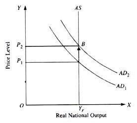
Here, OYF is the level of potential national output corresponding to the full-employment of labour (with a given natural rate of unemployment); AS is aggregate supply curve. AD1 is the aggregate demand curve which intersects the aggregate supply curve AS which gives price level equal to P1. Suppose Government takes up an expansionary monetary policy to increase output and employment. Thus, aggregate demand curve shifts to AD2. Rational expecta-tions theory believes that, people (i.e., labourers, firms, consumers, lenders) correctly anticipates this expansionary policy which causes inflation in the economy and they will take up correct measures to protect themselves against this inflation. This leads to demand for higher wages by workers and get it granted resulting in rise of prices of the products. All these increases take place immediately. Hence, expansionary policy just raises the price level keeping the natural rate of unemployment unchanged. The levels of real national product and employment, wage rate, interest rate, levels of investment and consumption remains un-changed.

People’s anticipations or expectations of inflation and their decision making corresponding to expansionary monetary policy nullify the intended effort by the Government. It is due to this anticipation of inflation by the people and quick upward adjustments made in wages, interest etc., by them that the price level instantly rises from P1to P2, leaving the level of output Q remaining constant.

Therefore, according to the rational expectations theory, aggregate supply curve is a vertical straight line i.e. there is no trade off between inflation and unemployment and downward-sloping Phillips curve does not exist.

Conclusion on Phillips Curve and the Relationship between Inflation and Unemployment

If the economy is operating below full capacity, a significant increase in aggregate demand will cause a reduction in unemployment and higher inflation. Thus, there can be a tradeoff between unemployment and inflation in the short run. However, there is a disagreement on the validity of the policy for the long-run.

In an ideal world, policy makers will aim for low inflation rate and low unemployment rate but to achieve this, the economic growth needs to be sustainable and supply side policies to reduce cost-push inflation and structural unemployment.

Get Online Macroeconomics Homework Help with our Tutors

Get fast, reliable and affordable online homework help service from AssignmentHelp.net’s online Economics tutors for microeconomics, macroeconomics, economics for managers, business economics and more. Whether it is a homework assignment related to Phillips curve or problem set based on rational expectations and adaptive expectations or it is any macroeconomics term paper related to fiscal policy, monetary policy and related topics; Assignmenthelpnet’s online macroeconomics tutors are your best bet.