Differential Equations

Question 4

Part (a)

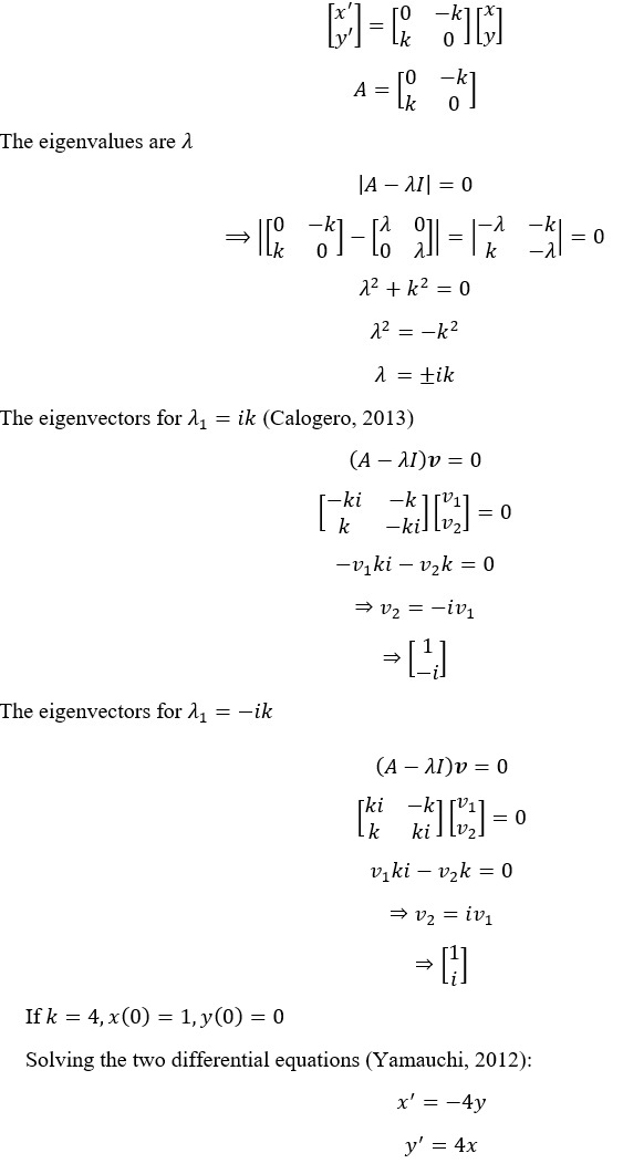
The information given implies that:

dx/dt∝-y,x decreases at a rate proportional to y

dy/dt∝x,y increases at a rate proportional to x

The constant of proportionality is the same,k for the two equations (Balamuralitharan, 2018): Therefore the system of differential equations are (Bird, 2017):

x^'=dx/dt=-ky

y^'=dy/dt=kx

In matrix form:

Using MATLAB we get:

Q4a:Obtaining eigenvalues and eigenvectors

syms k v1 v2

A=[0 -k; k 0];

Eigenvalues_Q4a=eig(A) %finding eigenvalues

[Eigenvectors_Q4a,DiagMat]=eig(A) %finding eigenvectors

Eigenvalues_Q4a =

 -k*1i

k*1i

Eigenvectors_Q4a =

[ -1i, 1i]

[ 1, 1]

DiagMat =

[ -k*1i, 0]

[ 0, k*1i]

Q4b: Solving the system of ODE

syms x(t) y(t)

%defining the odes

ode1=diff(x,t)==-4*y;

ode2=diff(y,t)==4*x;

odee=[ode1,ode2];

%defining the initial conditions

cond1=x(0)==1;

cond2=y(0)==0;

cond=[cond1,cond2];

%solving the ODEs using dsolve()

soln=dsolve(odee,cond);

x=soln.x;

y=soln.y;

% plotting x(t) and y(t)

t1=0:0.001:5;

figure(1)

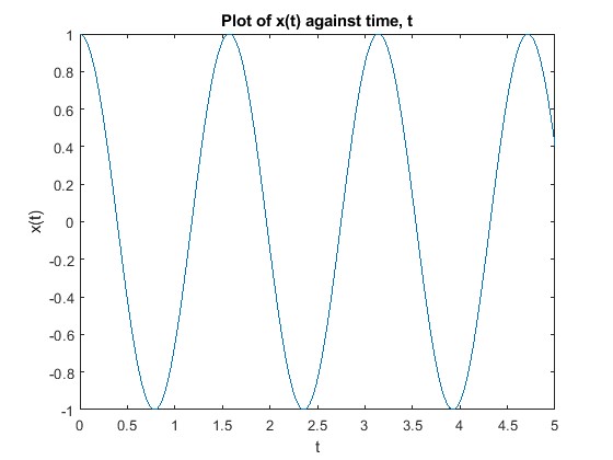
plot(t1,subs(x,t,t1))

xlabel("t")

ylabel("x(t)")

title("Plot of x(t) against time, t")

figure(2)

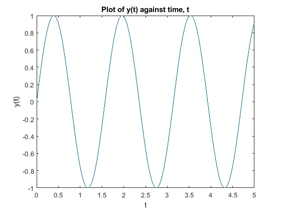
plot(t1,subs(y,t,t1))

xlabel("t")

ylabel("y(t)")

title("Plot of y(t) against time, t")

Question 1

Part a:

Let: (Shiwnarain, 2017)

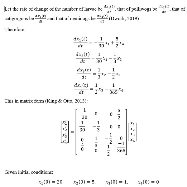
x₁ (t)be the number of larvae at time t

x₂ (t) be the number of polliwogs at time t

x₃ (t) be the number of catigorgons at time t

x₄ (t) be the number of demidogs at time t

MATLAB code and graphs (Magrab et al., 2010)

Q1a: System of ODEs

syms x1(t) x2(t) x3(t) x4(t)

%defining the differential equations

% x1---larvae

% x2---polliwogs

% x3---catigorgons

% x4---demidogs

eqn1=diff(x1,t)==-1/30*x1+5/2*x4;

eqn2=diff(x2,t)==1/30*x1-1/3*x2;

eqn3=diff(x3,t)==1/3*x2-1/2*x3;

eqn4=diff(x4,t)==1/2*x3-1/365*x4;

odee1=[eqn1,eqn2,eqn3,eqn4];

%defining the initial conditions

condi1=x1(0)==20;

condi2=x2(0)==5;

condi3=x3(0)==1;

condi4=x4(0)==0;

condi=[condi1,condi2,condi3,condi4];

% solving the ODEs

soln1=dsolve(odee1,condi);

% obtaining the values of x1, x2, x3 and x4 from the solution

x1=vpa(soln1.x1,3);

x2=vpa(soln1.x2,3);

x3=vpa(soln1.x3,3);

x4=vpa(soln1.x4,3);

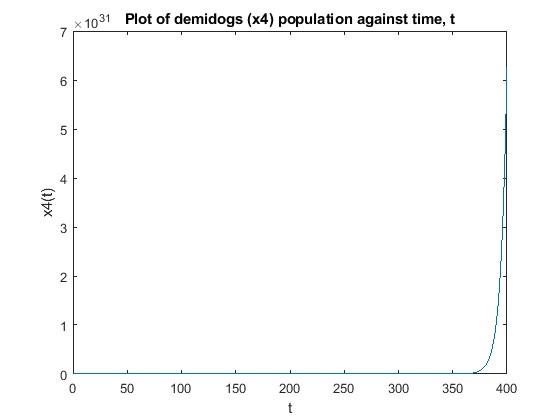
% plotting x4---demidogs against time

t2=0:1:400;

figure (3)

plot(t2,subs(x4,t,t2))

xlabel("t")

ylabel("x4(t)")

title("Plot of demidogs (x4) population against time, t")

disp("The number of demidogs after 7 days")

Demidogs_7=uint64(abs(subs(x1,t,7)))

disp("The number of demidogs after 30 days")

Demidogs_30=uint64(abs(subs(x1,t,30)))

disp("The number of demidogs after 365 days")

Demidogs_365=uint64(abs(subs(x1,t,365)))

Warning: Imaginary parts of complex X and/or Y arguments ignored

The number of demidogs after 7 days

Demidogs_7 =

uint64

70

The number of demidogs after 30 days

Demidogs_30 =

uint64

4970

The number of demidogs after 365 days

Demidogs_365 =

uint64

18446744073709551615

Part b

The coefficient matrix from part (a) is:

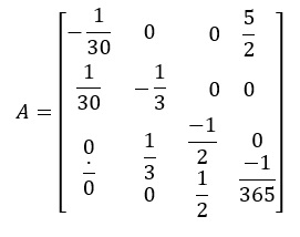
MATLAB Code for eigenvalues of A:

Q1b: Eigenvalues of coefficient matrix from A

A=[-1/30 0 0 5/2; 1/30 -1/3 0 0; 0 1/3 -1/2 0; 0 0 1/2 -1/365];

Eigenvalues_Q1b=eig(A)

Eigenvalues_Q1b =

-0.6273 + 0.0000i

-0.2118 + 0.2775i

-0.2118 - 0.2775i

0.1815 + 0.0000i

References

Balamuralitharan, S. (2018). MATLAB Programming of Nonlinear Equations of Ordinary Differential Equations and Partial Differential Equations. International Journal of Engineering & Technology, 7(4.10), 773. https://doi.org/10.14419/ijet.v7i4.10.26114

Bird, J. (2017). Higher Engineering Mathematics, 8th Ed. Routledge.

Calogero, F. (2013). A linear second-order ODE with only polynomial solutions. Journal of Differential Equations, 255(8), 2130–2135. https://doi.org/10.1016/j.jde.2013.06.007

Dwork, B. (2019). On Systems of Ordinary Differential Equations with Transcendental Parameters. Journal of Differential Equations, 156(1), 18–25. https://doi.org/10.1006/jdeq.1998.3593

King, A. C., & Otto, S. R. (2013). Differential equations : linear, nonlinear, ordinary, partial. Cambridge University Press.

Magrab, E. B., Shapour Azarm, & College, M. (2010). An engineer’s guide to MATLAB. Prentice Hall.

Shiwnarain, M. (2017). Life Cycle Of A Butterfly: Stages Of Life. Science Trends. https://doi.org/10.31988/scitrends.3973

Yamauchi, Y. (2012). Life Span of Positive Solutions for the Cauchy Problem for the Parabolic Equations. International Journal of Differential Equations, 2012, 1–16. https://doi.org/10.1155/2012/417261