Kurtosis and normality library agostino skewness test data ess skew

Analysis:
First, we load the kidscalories dataset and use the functions str to look at the data and study it in detail.

> library(readxl)
> library(moments)
> #Read the dataset kidscalories
> kidc <- read_excel("kidscalories.xls")
> View(kidc)
> str(kidc)
Classes ‘tbl_df’, ‘tbl’ and 'data.frame': 47 obs. of 2 variables: $ helpedinprep : num 1 1 1 1 1 1 1 1 1 1 ...

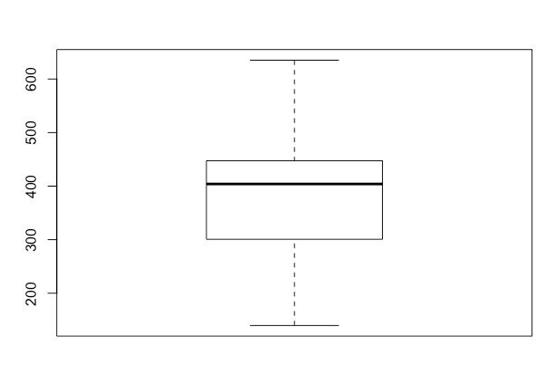
> hist(kidc$calorieintake)

> agostino.test(kidc$calorieintake)
D'Agostino skewness test

data: kidc$calorieintake
skew = -0.011821, z = -0.037082, p-value = 0.9704
alternative hypothesis: data have a skewness

Shapiro-Wilk normality test

data: kidc$calorieintake
W = 0.97936, p-value = 0.5663
The tests above shows that the data in question has negative skewness and evidence to light trails for normality. The p value that is 0.5663 which is higher than the threshold which means the distribution is close to normal.

We work with the Cholestoral dataset for this analysis. It gives us data on the change in cholesterol after a drug is taken by the patient

> library(readxl)
> library(moments)
> col <- read_excel("CholestoralData (1).xlsx")
> View(col)
> str(col)

We plot the density graphs for both the before and after column. Here we have two columns of important data and hence we will have to analyze the distributions of both before we step into the change from before to after.

> plot(density(col$Before))

> agostino.test(col$Before)

D'Agostino skewness test
data: col$Before
skew = 0.89653, z = 2.38360, p-value = 0.01714
alternative hypothesis: data have a skewness
> agostino.test(col$After)
D'Agostino skewness test
data: col$After
skew = 0.73814, z = 2.01770, p-value = 0.04362
alternative hypothesis: data have a skewness
> anscombe.test(col$Before)
Anscombe-Glynn kurtosis test
data: col$Before
kurt = 3.05270, z = 0.53771, p-value = 0.5908
alternative hypothesis: kurtosis is not equal to 3
> anscombe.test(col$After)
Anscombe-Glynn kurtosis test
data: col$After
kurt = 2.58600, z = -0.27481, p-value = 0.7835
alternative hypothesis: kurtosis is not equal to 3
> shapiro.test(col$Before)
Shapiro-Wilk normality test
data: col$Before
W = 0.91834, p-value = 0.00683
> shapiro.test(col$After)
Shapiro-Wilk normality test
data: col$After
W = 0.91706, p-value = 0.006231
We can see from the tests above that both the data are positively skewed and are not normally distributed. Hence, we normalize the curve and remove skewness for both.

> t.test(Bef, Aft, paired=TRUE, alternative='two.sided')

Paired t-test

Bartlett test of homogeneity of variances

data: After and margarine
Bartlett's K-squared = 0.93119, df = 1, p-value = 0.3346

3) EspressoData – three brew methods with a measure of the crème on the top. Find the method producing the most crème.

Analysis:

We start with tests to check the data for skewness, Kurtosis and normality.

> library(moments)
> agostino.test(ess$cereme)
D'Agostino skewness test
data: ess$cereme
skew = 0.54679, z = 1.32790, p-value = 0.1842
alternative hypothesis: data have a skewness
> anscombe.test(ess$cereme)
Anscombe-Glynn kurtosis test
data: ess$cereme
kurt = 2.33130, z = -0.58842, p-value = 0.5563
alternative hypothesis: kurtosis is not equal to 3
> shapiro.test(ess$cereme)
Shapiro-Wilk normality test
data: ess$cereme
W = 0.92201, p-value = 0.04414
To correct the Kurtosis and normalizing the curve,
> c1 <- log(ess$cereme)
> plot(density(c1))