BUS 450 Senior Capstone Business Penn Foster College
Case 2: Motomart
Introduction
cost accounting textbook coverage of cost behavior and variable costing using real-world cost data and an auto-industry-accepted cost driver. Unlike textbook problems, this data is real. It won’t necessarily produce a clear solution when you attempt to analyze cost behavior and apply scatter-plot, high-low, and regression methods to separate mixed costs into their fixed and variable components. This case also illustrates that financial accounting decisions and methods can have an influence on cost accounting and managerial applications and decision.
Objective
When you complete this case, you’ll be able to
- Explain the importance of accrual accounting and proper
- application of the matching principle for the computation
- of contribution margins and break-even points
- Apply knowledge of generally accepted accounting
- principles (GAAP) to a specific real-world example
- Integrate statistical analyses and scatter plots, line
- graphs, and regression to determine the reliability of
- financial information prepared for external use
- Use analytical review procedures to examine a firm’s
- financial statements
- Apply critical-thinking skills to real-world
- business circumstances
CASE BACKGROUND
This case is based on real financial data provided by a retail automobile dealership (Motomart) seeking to relocate closer to an existing retail dealership. You’ll examine the mixed cost data from Motomart and apply both high-low and regression to attempt to separate mixed costs into their fixed and variable components for break-even and contribution margin computations. You’ll find that the data is flawed because Motomart was a single observation in a larger database. Don’t attempt to correct the data (e.g., remove outliers or influential outliers). You’ll be producing a scatterplot and apply high-low and regression methods to the extent practicable and writing a summary report of the findings.
Motomart operates a retail automobile dealership. The manufacturer of Motomart products, like all automobile manufacturers, produces forecasts. It has long been an industry practice to use variable costing-based/break-even analyses as the foundation for these forecasts, to examine their cost behavior as it relates to the new retail vehicles sold (NRVS) cost driver. In preparing this financial information, a common financial statement format and accounting procedures manual is provided to each retail auto dealership.
The dealership is required to produce monthly financial statements using the guidelines provided by this common accounting procedures manual, and then furnish these financial statements to the manufacturer. General Motors, Ford, Nissan, and all other automobile manufacturers employ similar procedures manuals.
The use of a common format facilitates the development of composite financial statements that can be used to estimate costs and produce financial forecasts for future or proposed retail dealership sites (Cataldo and Kruck 1998). Zimmerman (2003) suggests that as many as 77 percent of manufacturers divide costs into variable and fixed components, and that managers arrive at these estimates by classifying individual accounts as being primarily fixed or primarily variable (67).
For this case, you’ll examine mixed costs as defined by the manufacturer. Using the scatterplot, high-low, and regression methods, separate these mixed costs into their fixed and variable components. The data is problematic, and a clear solution won’t exist. Don’t attempt to correct the data by removing outliers, but make observations based on any patterns you observe. The case will expose you to actual data and require you to summarize your findings, including any conclusions you’re able to reach and why the financial data makes it impossible to separate the mixed costs into their fixed and variable components.
Motomart: A Litigation Support Engagement
The Motomart case evolved from a litigation support engagement. The lead author of this case was hired to analyze the data and provide expert testimony. His report and testimony was made available to the public (for a fee to cover reproduction costs). A broad description of the relevant points for the Motomart case follows.
Motomart wanted to move their retail automobile dealership, blaming their location for declining profits and increasing losses. They provided financial projections, using variable costing, to show that after relocation both Motomart and the existing dealership would be profitable. They created these financial projections using a database provided by the manufacturer, which included all North American retail automobile dealerships. Motomart was one of the observations or retail automobile dealerships included in the database used to create these financial projections. You’ll be examining portions of Motomart’s historical financial data.
The relocation site was quite close to the existing dealership (which we’ll refer to as Existing Dealer), and Existing Dealer felt that, if the relocation was permitted, one or both of the dealerships would fail to break even and eventually go bankrupt, leading to poor service, or what the industry refers to as “orphaned” owners of these automobiles.
Antitrust laws provided Existing Dealer with the means to block the relocation requested by Motomart, but only if it could prove that the relocation wasn’t in the best interest of the consuming public. Generally, the only way to prove this is to prove that there’s simply not enough business for both retail automobile dealerships to break even (or generate a reasonable return on investment, given the risks associated with the industry). Again, the manufacturer, in support of the proposed Motomart relocation, supplied financial projections showing that both retail automobile dealerships would be profitable after the relocation.
The expert witness hired to investigate the merits of the relocation was given the Motomart data, but not the entire database that included the Motomart data. The Motomart data was in such poor form that it wasn’t possible to produce a financial forecast. An alternative forecast, not included in this case, was produced. This alternative forecast did not support the relocation of Motomart to a site closer to Existing Dealer. The alternative forecast showed that the market simply couldn’t support two retail automobile dealerships. The implication was that, as the weaker of the two dealerships, Motomart was losing business to Existing Dealer. In conclusion, the relocation request by Motomart was denied.
Income and Expense Data
The following tables give you information such as income statements, semi-fixed expenses, and salaries for Motomart. Look for unusual entries or discrepancies in their records and, where you can, note the cause of the problems.
Table 3 summarizes financial and cost driver information produced by Motomart, where new retail vehicles sold (NRVS) is the cost driver. The account classification method has resulted in three cost behavior classifications: variable, semi-fixed, and fixed costs. Semi-fixed is the automobile industry-specific term used for mixed costs. We’ll assume that Motomart’s classifications of variable costs (VCs) and fixed costs (FCs) are correct, and focus our analysis on Motomart’s semi-fixed or mixed costs.
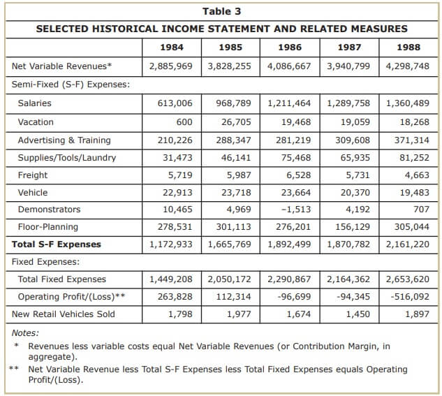
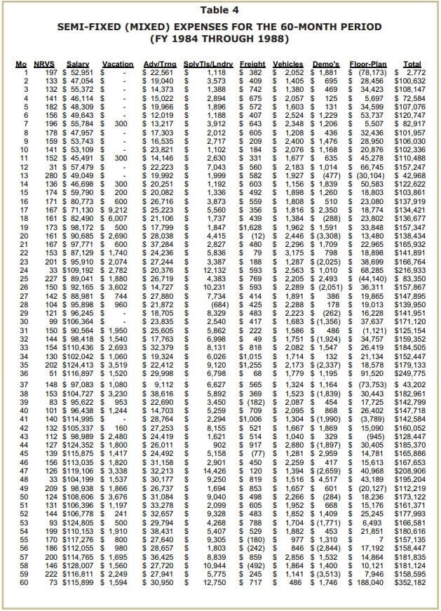
Table 4 provides five years of monthly data (N=60) for NRVS and the related semi-fixed or mixed cost measures. Semifixed costs were significant. Recall that they ranged from nearly $1.2 million for calendar and fiscal year (FY) 1984 to almost $2.2 million for FY 1988 (see Table 3).
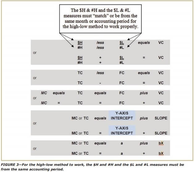
Recall the cost function applying to the high-low and regression methods, which are provided in a variety of forms, depending on the texts you used in your previous math, economics, or accounting Assignments. Figure 3 is a brief outline of the high-low and regression methods.
Preparing Graphs
The single cost driver and nonfinancial measure in Table 4 is new retail vehicles sold (NRVS or X in the above cost function). There are eight financial measures (salary; vacation; advertising and training; supplies, tools, and laundry; freight; vehicles; demonstrators; and floor-planning [also known in the automobile retail industry as interest expense relating to new car inventory]), as well as a total (aggregate measure) provided for all eight financial measures (or the Y in the above cost function).
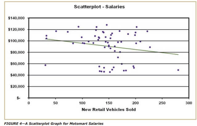
Using NRVS, the only available cost-driver, use Excel to prepare nine separate scatter plots and cost function-based trend lines and nine separate line graphs for each of the financial measures provided in Table 4. See Figure 4 and Figure 5 for a examples of completed graphs for salaries.
Now examine, on a preliminary basis, the pattern or trend (or lack thereof) for each of the “X” (NRVS) and “Y” (financial measure) data pairs and consider the following questions:
- You’re observing these data pairs for a 60-month period (i.e., five years); are any annual or other seasonal patterns or trends immediately apparent?
- Do the slopes of the trend lines (i.e., variable costs) make sense?
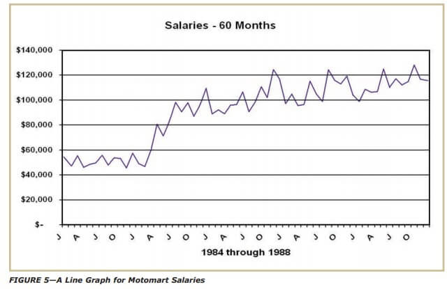
In the case of salaries (see Figures 4 and 5), there’s no apparent trend or pattern. It’s odd that salaries decrease as NRVS increases—in fact, this doesn’t make any sense. However, it’s consistent with the high-low results, which also didn’t make sense. But remember, since this data came from Motomart, the firm attempting to relocate, it’s real and from an actual litigation support engagement (not a textbook problem), so it won’t necessarily work out perfectly.
The cost equation in Table 5 shows fixed costs (FC) at $106,866.00 and variable costs to be used to “reduce” total costs (TC) by $110.10 per NRVS. Compare the salary figures and coefficients (in bold type) to Figure 4. Notice that if you extended the trend line in Figure 4, it would hit the y-axis intercept at $106,866.00 (the fixed cost). Also notice that the R-squared (R-sq) measure in Table 5 equals 4.1 percent.
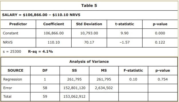
Your math and statistics Assignments probably reviewed the use of the t-statistic, overall F-statistic, and related p-values, as well as some of the other measures presented here. Our application is a very simple one, so we’ll focus on only the R-squared measure. The other measures are provided in this example only for completeness.
Because the high-low technique didn’t work, it makes sense that the regression technique wouldn’t work well, either. Therefore, the results for high-low and regression are consistent. The advantage of the regression technique is that it mathematically quantifies the level of the problem or difficulty with the data. In this case, one of simple regression, the R-squared measure tells the story. Still focusing on the salaries example in Figure 5, the R-squared measure tells us that only 4.1 percent of the total or mixed or semi-fixed cost is explained by NRVS. This means that that cost equation developed from this historical data isn’t helpful in predicting future costs, as nearly 96 percent of the cost behavior, through use of this equation, remains unexplained.
REQUIREMENTS
Operating Profits and Semi-Fixed Expenses
Step 1
First, using Tables 3–5, note the pattern of operating profits (or losses) over the five-year period. Then focus only on the semi-fixed expenses contained in Table 3. Do any amounts appear to be odd? Next, briefly comment on the five-year pattern or trend for operating profit/loss measures. You should be able to respond to this step in a few well written sentences.
Step 2
Focus only on the detailed semi-fixed expense contained in Table 4. Are there any unusual or odd patterns you might note in this detailed financial data? There are eight expense items. About five of the eight should immediately catch your attention. You should be able to respond to this requirement in a few well-written sentences. Briefly comment on only the most obvious or apparent measures or patterns, by expense item.
Step 3
Identify the high and low measures in each column, just as you would in preparation for application of the high-low method or technique. For example, in Table 4 the high measure for the cost driver (NRVS) is 280 NRVS in month 13 and the low measure is 31 NRVS in month 12. Repeat this process for each of the eight separate semi-fixed expense columns and also for the total expense column. (You could transfer the figures to Excel to use the maximum and minimum functions to assist you in identifying the high and low measures [N=60] for each of the ten columns.)
After the high and low measures have been identified in each column, try to match each expense column’s high and low measure, separately, to the highs and lows identified in the NRVS column. They won’t match. Don’t try to correct the data, but comment on the potential for application of the high-low technique. What happens when the high and low activity level doesn’t match the high and low expense measure? Does this prevent you from correctly applying the high-low technique?
Don’t overanalyze this data, because there’s a problem with it and you don’t have sufficient information to correct it. Merely summarize your observations and unsuccessful attempts to match the high and low NRVS months (identified above), separately, with each of the high and low expense measure months. You should be able to do this in a very few well written sentences.
Finally, summarize your findings with respect to the application of the high-low method to separate mixed costs into their fixed and variable components or the development of a cost equation.
Step 4
Use Table 6 to compute the cost equations and R-squared measures for each of the remaining eight expenses and total expenses. Notice that there’s a computed total requirement in the table. This just means that you must total these two columns and compare the computed totals to the Excelgenerated measures in the row below. In effect, you’re being asked to comment on whether the separate cost formulas are “additive.”
| Table 6 | ||||
|---|---|---|---|---|
| Column | Expense | FC | VC | r-sq |
| 1 | Salaries | $106,866 | –$110 | 4.10% |
| 2 | Vacation | |||
| 3 | Advertising and training | |||
| 4 | Supplies/tools/laundry | |||
| 5 | Freight | |||
| 6 | Vehicles | |||
| 7 | Demonstrators | |||
| 8 | Floor planning | |||
| Computed total | ||||
| 9 | Total | |||
Complete the cost equations for the table. Use the R-squared as the single measure of “goodness of fit.” Don’t attempt to improve your results with the elimination of “outliers” or “influential outliers.” As you complete Table 6, answer the following questions:
- What problems did you encounter?
- Are the R-squared measures high or low?
- Are the slopes negative or positive?
- Are your conclusions consistent with those from the
- high-low effort?
Step 5
Summarize your findings on a single page (250 words or less, double-spaced). Can the Motomart data be used to prepare a reliable financial forecast? Why or why not? If Motomart is included in the very large database used to prepare the financial forecast that supports the relocation of Motomart closer to Existing Dealer, what concerns might present themselves with respect to the remainder of the database used for this forecast? Would you rely on this forecast?
It’s common for businesses to keep poor financial records most of the year, because many are trying to reduce the cost of financial record keeping (e.g., the salary of a CPA is higher than that of a bookkeeper). Then, at the year’s end, these businesses employ a CPA or accounting firm to make adjusting journal entries to correct data for the twelfth months of the year, only to reverse the adjusting journal entries immediately after the annual financials are prepared.
Examine your graphics to identify any seasonal (12-month) patterns. Do any exist? Is there evidence to suggest that the process described above was being employed by Motomart?


